Macroeconomic Policy\(:\) The AD/AS/MP Model
Week 09
April 28, 2025
1. The Goals of Macroeconomic Policy
The Divine Coincidence
- Short-term macroeconomic policy has 2 fundamental objectives:
- To stabilize economic activity (GDP) and the level of unemployment.
- To stabilize inflation at a relatively low value.
. . .
\[Y=Y^P, \quad \text { then } \quad U=U^n, \quad \text { and } \quad \pi=\pi^e=\pi_{-1}\]
. . .
- Some economists call this situation the divine coincidence, sarcastically, as something ideal but unattainable 1
Inflation Rate Target
All central banks in advanced countries have an optimal value for inflation they want to achieve. This is called the inflation target:\[\color{blue}{\pi^{_T}}\]
. . .
\(~~~~~~~~~~~~~~~~~~~~~~~~\)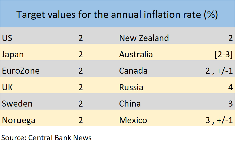
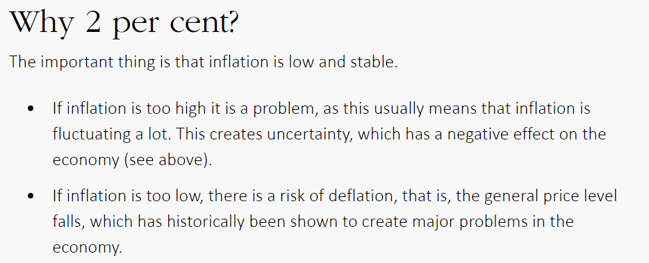
Why \(2\%\) Inflation?
. . .
According to the Swedish Central Bank (Sveriges Central Bank):
. . .
2. Stabilization Policy
Long-Run = Short-Run Equilibrium
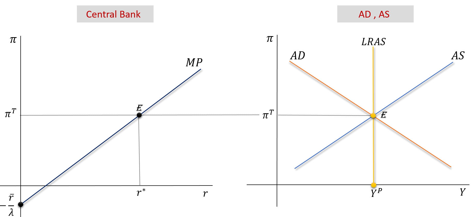
The central bank sets \(i\) such that \(r\) will lead to the “divine coincidence”: \(Y=Y^P \ , \ U=U^n \ \ , \ \pi=\pi^{_T} \ \). See an animated version here
3. Aggregate Demand Shocks
Soft Reaction by the Central Bank
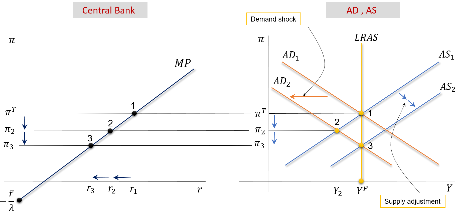
Consider that \(\overline{A} \downarrow\). Then \(\pi \downarrow\), the central bank reduces \(r\) and accepts \(\pi<\pi^{_T}\). See the animated version here
Previous Slide’s Details: Read at Home
Autonomous Demand decreases for some reason. It can be caused by a government decision \((T \uparrow,G \downarrow )\), a decrease in NX, or any other change in \(\overline{A}\).
The AD function moves from AD1 to AD2 and the economy moves to point 2. At point 2, we have an economic recession \(\left(Y_2<Y^P\right)\), and an inflation rate below the target \(\left(\pi_2<\pi^{_T}\right)\).
At point 2, as inflation has fallen, the CB lowers the interest rate interest rate \((r_1 \rightarrow r_2)\). At this point, since we have a recession, by the supply self-correcting mechanism, inflation will decrease over time. The AS function moves from AS1 to AS2.
The new equilibrium point will be at point 3 . We will have: \[ Y=Y^P, \quad \pi=\pi_3<\pi^{_T}, \quad r=r_3 \]
Soft vs Aggressive Response By the CB
- The Central Bank (CB) decisions in the previous figure have an implicit fact: the CB accepts the new value of inflation as the new equilibrium: \(\pi^{_T}=\pi_3\).
The textbook says that “There is no policy response” in this case, which may confuse more than elucidate. There is a policy response by the CB because it changes interest rates: \(r_1 \rightarrow r_2 \rightarrow r_3\). The point is that its response is “soft”, rather than “aggressive”. Understanding the difference between these two reactions is crucial.
- So, what happens if the CB does not accept a change in its initial target value for inflation \(\left(\pi^{_T}\right)\) ? It will have to implement an aggressive monetary policy by imposing a radical cut in interest rates, not a gradual one.
- That will be the contents of next slide.
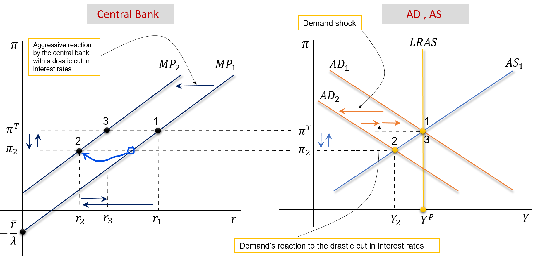
Aggressive Reaction by the Central Bank
Consider that \(\overline{A} \downarrow\).Then \(\pi \downarrow\), the central bank drastically \(r \downarrow\) and forces \(\pi \rightarrow \pi^{_T}\). See the animated version here
Previous Slide’s Details: Read at Home
The only difference between the central bank’s aggressive response and its soft one is related to the level of interest rate reduction it imposes in both cases.
Soft response: The central bank imposes a small reduction in the interest rate in order to accommodate the reduction in inflation. The impact on demand is small.
Aggressive response : the central bank does not want the economy to reach point 2. To this end, when there is a reduction in autonomous demand \((\overline {A})\), it drastically cuts the interest rate, stimulating Consumption, Investment, and Net Exports, which leads to a shift in the AD curve to the initial position.
The new long-run equilibrium is now characterized by: \[ Y=Y^P, \quad \pi=\pi^{_T} \quad \text{and} \quad r=r_3 \]
4. Permanent Aggregate Supply Shocks
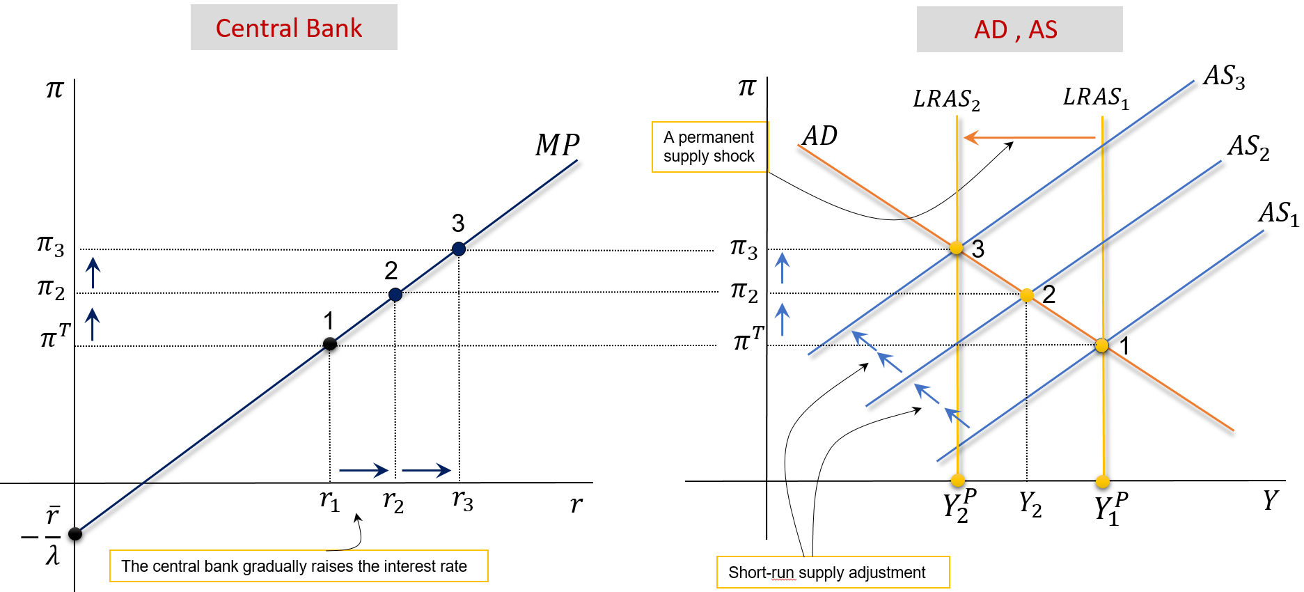
Permanent AS Shock: Soft Response
Suppose international oil prices increase and don’t go down. Then \(\pi \uparrow\), the central bank increases \(r\) and accepts \(\pi>\pi^{_T}\). See the animated version here
Previous Slide’s Details: Read at Home
There is a negative supply shock, for example, caused by an increase in the price of oil, after which, oil prices remain constant.
This increase causes a shift from LRAS1 to LRAS2. The new equilibrium point is at point 2. This point is obtained because the economy is in an economic boom at 1 , since \(\left(Y_1^P>Y_2^P\right)\), which causes inflation to increase over time. This process is described by the shift from AS1 to AS2.
From point 2, we move to point 3, for the same reason. Note that the central bank has been raising the interest rate in order to keep up with the increase in inflation.
Point 3 will be the new long-run equilibrium point if the central bank accepts a higher value \(\pi^{_T}\) : \[ Y=Y_2^P \ , \quad \pi=\pi_3=\pi_3^{_T} \ , \quad r=r_3 \]
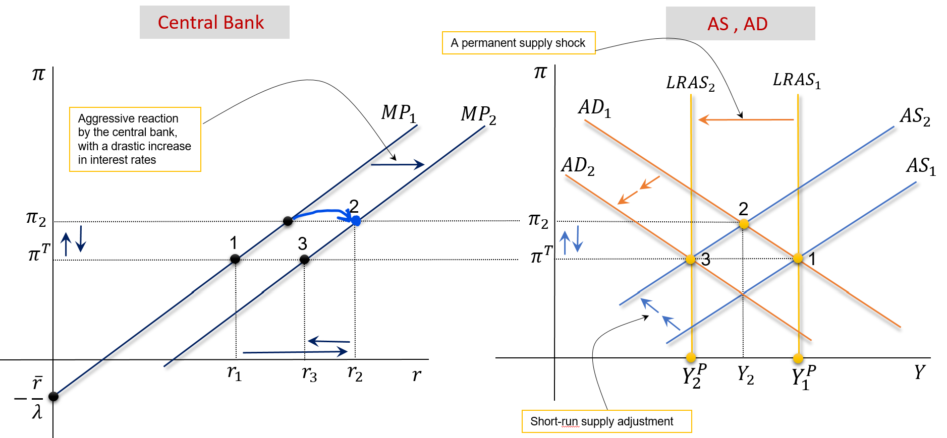
Permanent AS Shock: Aggressive Response
Suppose oil prices increase and don’t go down. Then \(\pi \uparrow\), the central bank drastically increases \(r\) to avoid \(\pi>\pi^{_T}\). See the animated version here
Previous Slide’s Details: Read at Home
The central bank does not want the economy to reach point 3 , in the case where the response was soft.
To this end, when inflation increases, the central bank drastically raises the interest rate. This increase can be seen by the movement of MP1 to MP2, which leads to a reduction in Consumption, Investment, and Net Exports, generating a shift of the AD curve: AD1 to AD2.
The new long-run equilibrium will be characterized by: \[ Y=Y_2^P \ , \quad \pi=\pi^{_T} \ , \quad r=r_2 \]
The aggressive response by the central bank, in this case, led to the stabilization of both GDP and inflation.
5. Temporary Aggregate Supply Shocks
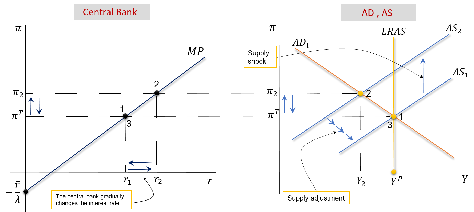
Temporary AS Shock: Soft Response
Suppose that oil prices increase temporarily \((\rho \uparrow)\). The CB softly reacts to the shock. See the animated version here
Previous Slide’s Details: Read at Home
This temporary increase does not cause any shift in LRAS. It does cause a temporary increase in inflation, displacing AS1 to AS2.
The new equilibrium point is 2 . At this point, the economy is in a recession, since \(\left(Y_2<Y^P\right)\), which will force inflation to decrease over time. This process is described by the gradual shifts from AS2 to AS1, until the initial point is reached.
Note that the central bank has been changing the interest rate in order to keep up with the changes in inflation.
Point 3 will be the new long-run equilibrium point if the central bank accepts a lower value for \(\pi^{_T}\) : \[ Y=Y_2^P, \quad \pi=\pi_3=\pi_3^{_T}, \quad r=r_3 \]
Temporary AS Shock: Aggressive Response
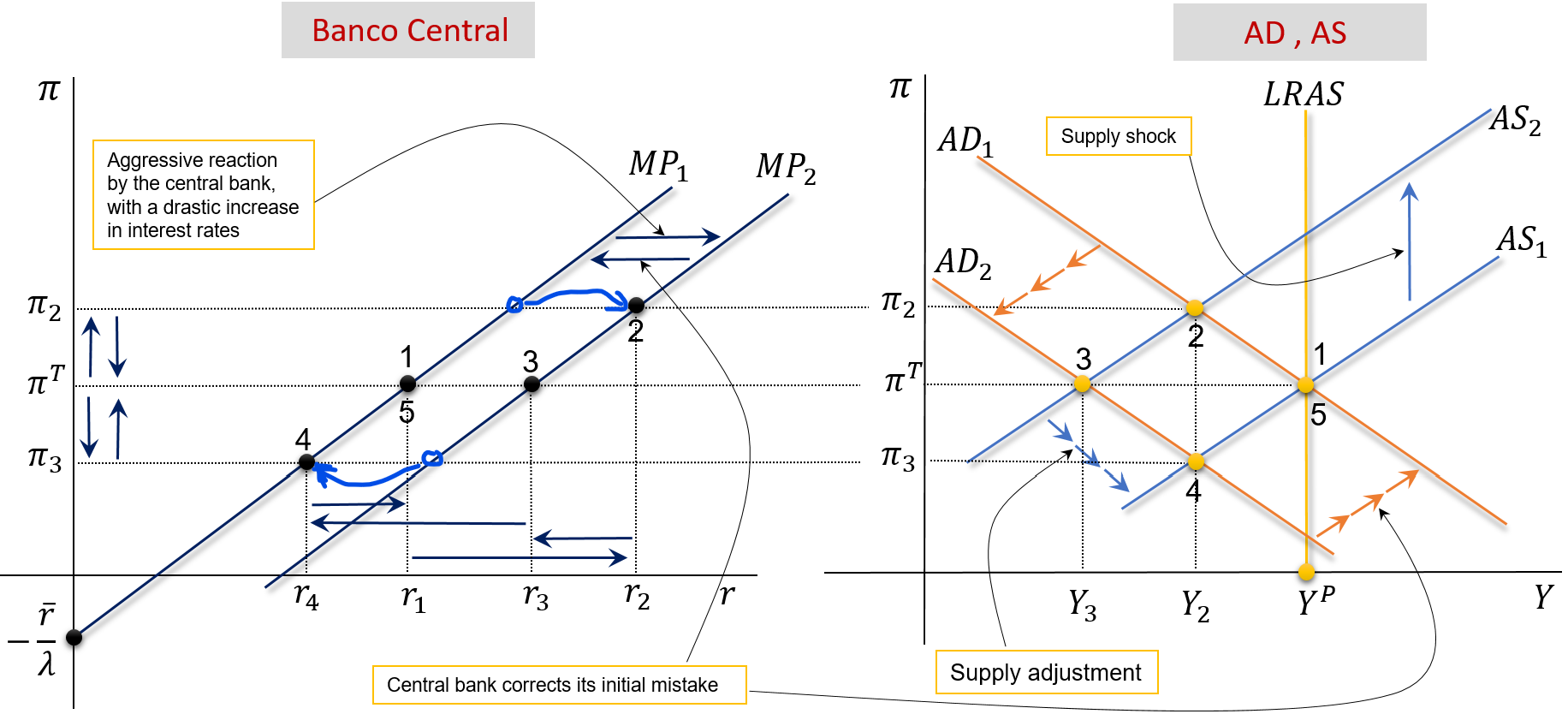
Suppose that oil prices increase temporarily \((\rho \uparrow)\). The CB aggressively reacts with a sharp increase in interest rates. See the animated version here
Previous Slide’s Details: Read at Home
The central bank makes the mistake of responding aggressively to a temporary supply shock.
In point 2, we already know how this works: see the previous case. Except that now in point 2, the central bank decides to raise the interest rate by a lot. This causes MP1 \(\rightarrow\) MP2 and AD1 \(\rightarrow\) AD2. We move on to point 3 .
At point 3, we have a big recession, which will lead to a reduction in inflation, leading to AS2 \(\rightarrow\) AS1. We are left at point 4 .
At this point, inflation is below the desired level ( \(\pi_3<\pi^{_T}\) ), and the central bank has no other remedy than to undo what it did at the beginning: now drastically reduce the interest rate. This shifts AD2 to AD1 and we end the process at point \(5(=1)\).
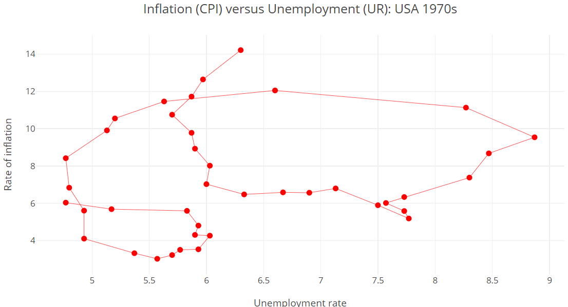
The central bank’s mistake has created a loop in inflation like in the 1970s.
Inflation Loops in the 1970s: USA
The Phillips Curve of the 1970s seems to confirm the circular movement of inflation seen in the previous figure (points: \(1,2,3,4,5\) ).
5. Readings
Readings
Read Chapter 13 of the adopted textbook:
Frederic S. Mishkin (2015). Macroeconomics: Policy & Practice, Second Edition, Pearson Editors.
Footnotes
Blanchard, O. and Galí, J. (2007). Real Wage Rigidities and the New Keynesian Model. Journal of Money, Credit and Banking, 39, 35-65.↩︎