The Macroeconomic Equilibrium\(:\) Aggregate Demand & Supply
Week 08
ModernMacro team
Instituto Universitário de Lisboa (ISCTE-IUL)
April 13, 2026
1. Recap: The AD & AS Curves
Recap the AD Curve
\[Y=m \cdot \overline{A}-m \cdot \phi \cdot(\overline{r}+\lambda \pi) \tag{AD}\]
where:
- \(\overline{A}=\overline{C}+\overline{I}-d \cdot \overline{f}+\overline{G}+\overline{N X}-c \cdot \overline{T} \quad\) (Autonomous Aggregate Demand)
- \(m=\frac{1}{1-c} \quad\) (demand multiplier)
- \(\phi=b+d+x \quad\) (parameter used to simplify notation)
- \(\lambda \quad\) (parameter)
AD: Movements-Along vs Shifts
\[ Y=m \cdot \overline{A}-m \cdot \phi \cdot(\overline{r}+\lambda \pi) \tag{AD} \]
A movement along the AD curve: \(\pi\) changes, everything else constant. \[ \pi \uparrow \ \Rightarrow \ r \uparrow \ \Rightarrow\ \ \{I \downarrow, C \downarrow, NX \downarrow\} \Rightarrow \ Y \downarrow \]
A shift in the AD curve : \(\pi\) constant, everything else changes. \[ \{\overline{A} \uparrow, \overline{r} \downarrow\} \quad \Rightarrow \quad Y \uparrow \]
Recap the AS Curve
\[ \pi=\underbrace{\pi^e}_{=\pi_{-1}}+\gamma\left(Y-Y^P\right)+\rho \tag{AS} \]
- For simplicity, suppose that \(\rho = 0\).
- The long-run equilibrium :
- \(Y = Y^P\) and \(\ \pi = \pi^e\) : the economy is at Potential GDP and inflation is stable.
- The short-run equilibrium :
- \(Y \neq Y^P\) and \(\pi \neq \pi^e\) : the economy is either in a recession or in a boom.
- A boom will force \(\uparrow \pi\); a recession will force \(\downarrow \pi\): self-correcting mechanism.
AS: Movements-Along vs Shifts
\[ \pi=\underbrace{\pi^e}_{=\pi_{-1}}+\gamma\left(Y-Y^P\right)+\rho \tag{AS} \]
A movement along the AS curve: \(Y\) changes, everything else constant. \[ (Y-Y^P) \uparrow \ \Rightarrow \ \text{economic boom} \ \Rightarrow \ \pi \uparrow \]
A shift in the AS curve : \(Y\) constant, everything else changes. \[ \rho \uparrow \ \Rightarrow \pi \uparrow \quad, \quad \pi^e \uparrow \ \Rightarrow \pi \uparrow \quad, \quad Y^P \uparrow \ \Rightarrow \pi \downarrow \]
2. The Macroeconomic Equilibrium: AD=AS
The Short-run Equilibrium: Derivation
\(~~~~~~~~~~~~~~~~\)The AD curve: \[ Y=m \cdot \overline{A}-m \cdot \phi \cdot(\overline{r}+\lambda \pi) \]
\(~~~~~~~~~~~~~~~~\)The AS curve: \[ \pi=\underbrace{\pi^e}_{=\pi_{-1}}+\gamma\left(Y-Y^P\right)+\rho \]
Insert the AS into the AD, and solve for \(Y\) (to simplify define: \(\varphi = m \phi \lambda \gamma\)):
\[Y = \frac{m}{1+\varphi}\overline{A} - \frac{m\phi}{1+\varphi}\overline{r} -\frac{m \phi \lambda}{1+\varphi}\pi^e + \frac{\varphi}{1+\varphi}Y^P - \frac{m \phi \lambda}{1+\varphi}\rho \tag{1}\]To obtain the solution for \(\pi\) insert eq. (1) into the AS curve and get: \[ \pi = \frac{m \gamma}{1+\varphi} \overline{A} - \frac{m \phi \gamma}{1+\varphi} \overline{r} + \frac{1}{1+\varphi}\pi^e - \frac{\gamma}{1+\varphi}Y^P + \frac{1}{1+\varphi}\rho \tag{2} \]
Fortunately, we have the computer to easily solve these two equations for us. Do not worry about these two equations.
The Short-Run Equilibrium Graphically
. . .
The textbook provides a graphical solution to the short-run equilibrium: \(Y=Y^*\) and \(\pi=\pi^*\).
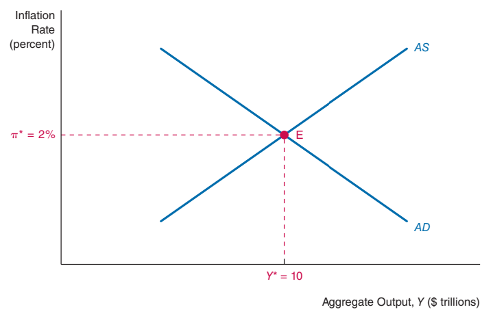
It may correspond to:
- a recession: \((Y<Y^P)\)
- a boom: \((Y>Y^P)\)
- a stable economy \((Y=Y^P)\)
The Short-run Equilibrium: \(Y<Y^P\)
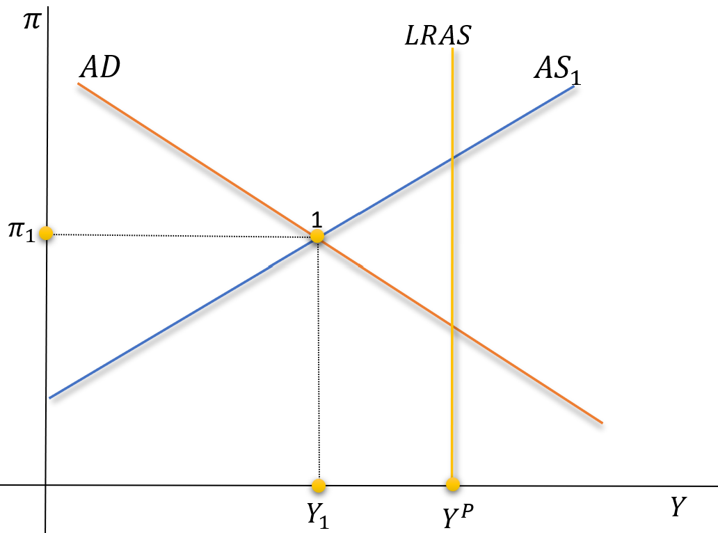
- Suppose the economy is initially in a recession, with \(Y_1<Y^P\).
- Click on any key
The Short-run Equilibrium: \(Y<Y^P\)

Logic:
- At point 1, \(Y_1 <Y^P\): recession
- This implies that \(\downarrow \pi\)
- If \(\downarrow \pi\), the AS has to come down
- Click on any key
The Short-run Equilibrium: \(Y<Y^P\)
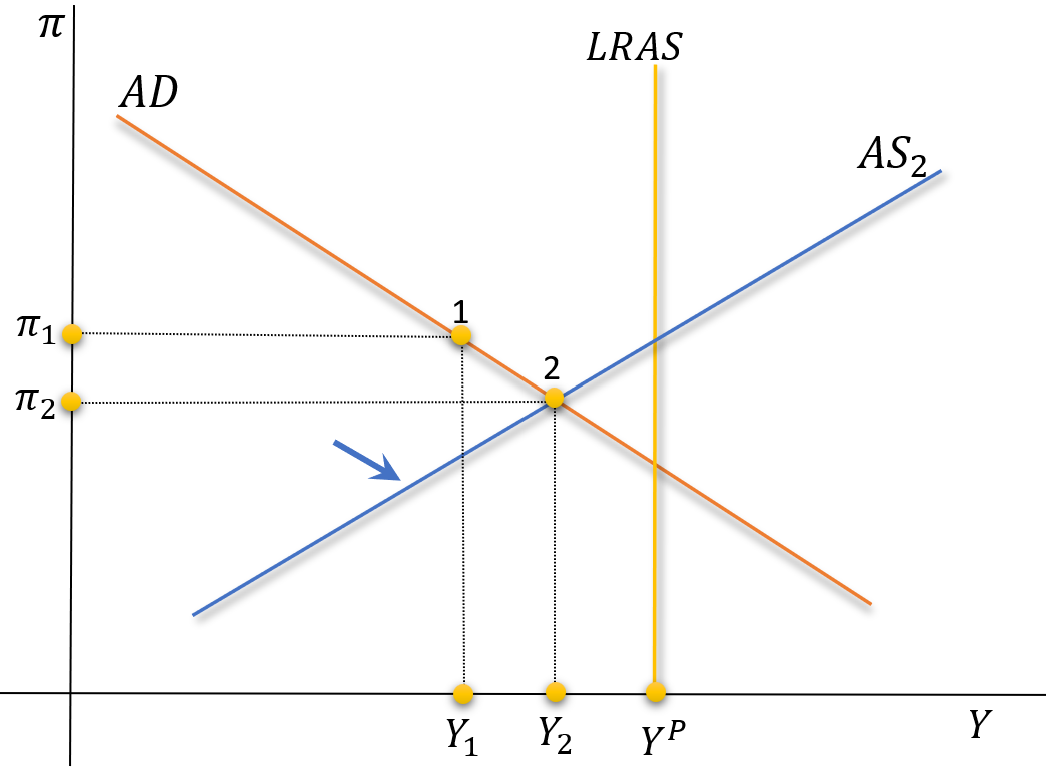
The recession is now smaller, but the economy is still in recession.

- At point 2, \(Y_2 <Y^P\): still in recession
- This implies that \(\downarrow \pi\)
- If \(\downarrow \pi\), the AS has to come down
- Click on any key
The Short-run Equilibrium: \(Y<Y^P\)
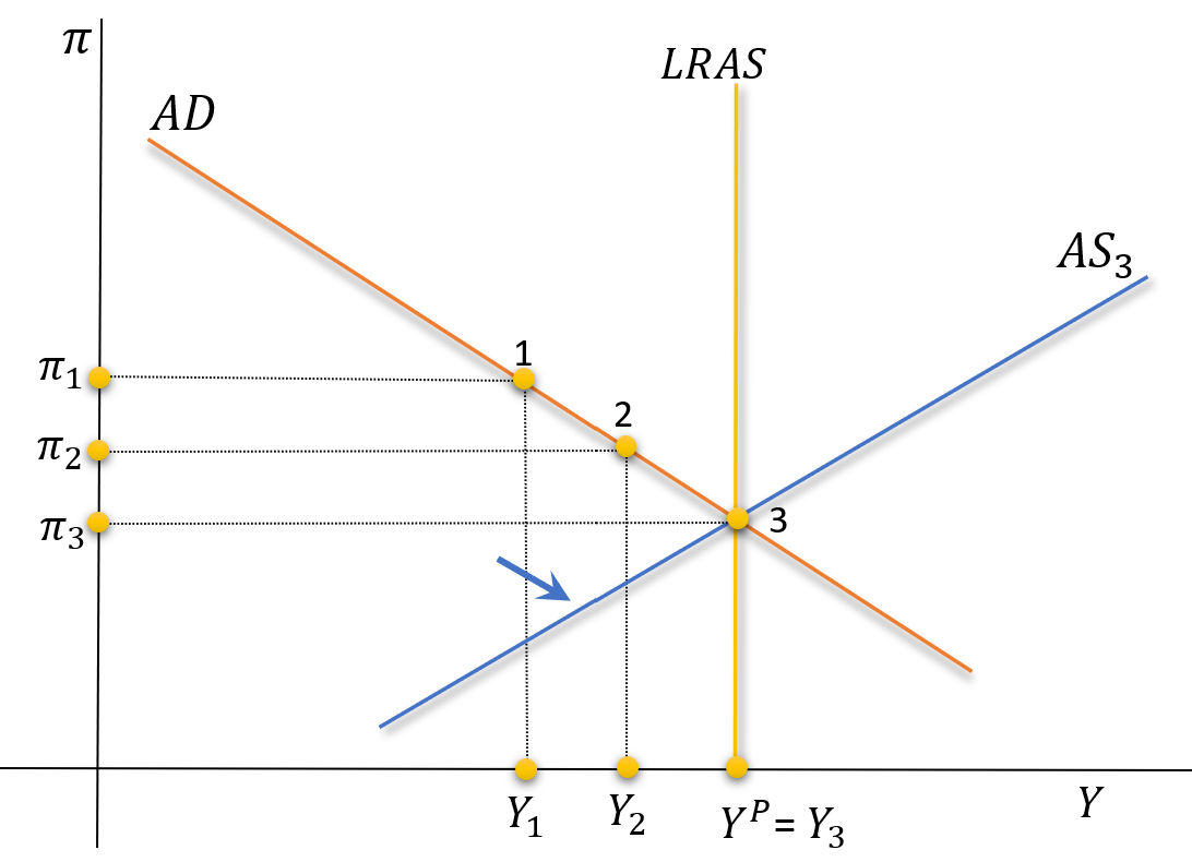
The recession is eradicated by the inflation self-correcting mechanism.

- At point 3, \(Y_3 =Y^P\): no recession
- This implies that \(\pi\) is stable
- If \(\pi\) is stable, the AS will remain in the same position
- At 3, we have a short and long term equilibria.
Previous Slide’s Details: Read at Home
Consider that \(Y_1<Y^P\) : point 1.
Unemployment is above the natural unemployment rate: \(U>U_n\) and wages decrease (Phillips curve).
Firms are forced to reduce their prices. The curve AS1 shifts to AS2 and inflation decreases below its initial level: \(\pi_2<\pi_1\).
In the next period, expectations of inflation \((\pi^e)\) are revised downward due to falling inflation and the AS continues to shift downwards from AS2 to AS3.
As long as we have \(Y<Y^P\), wages increases and inflation will continue to come down, causing the AS curve to shift downward: self-correcting supply mechanism.
The process repeats itself until \(Y=Y^P\), i.e., the economy reaches its long-run equilibrium, which occurs at point 3, with \(Y_3=Y^P\).
The Short-run Equilibrium: \(Y>Y^P\)
- Contrary to the previous case …
- Suppose the economy is initially in a boom, with \(Y_1>Y^P\).
- Click on any key
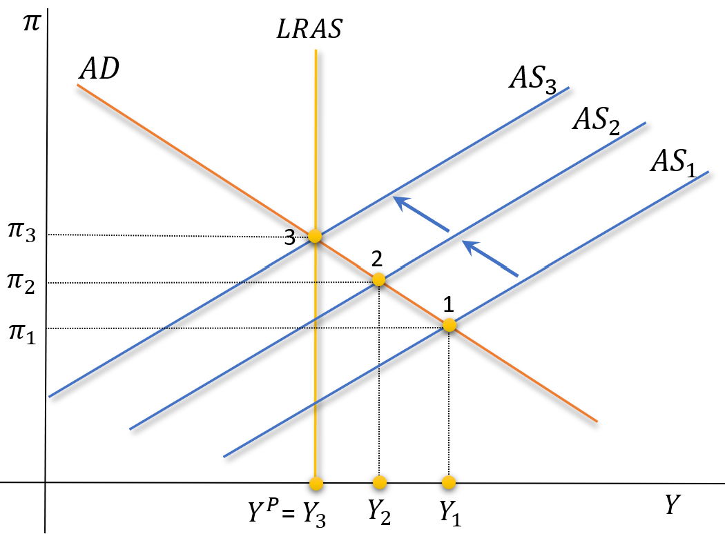
The Short-run Equilibrium: \(Y>Y^P\)
The self-correcting supply mechanism works with the same logic: the only difference is that now inflation is pressured to go up, not down.

- At point 1, \(Y_1 > Y^P\): boom
- This implies that \(\uparrow \pi\)
- If \(\uparrow \pi\), the AS has to go up
- AS only stops at point 3: \(Y_3=Y^P\)
- At 3, we have a short and long term equilibria.
Previous Slide’s Details: Read at Home
Consider that \(Y_1>Y^P\) : point 1.
Unemployment is below the natural unemployment rate: \(U<U_n\) and wages increase (Phillips curve).
Firms raise their prices. The curve AS1 shifts to AS2 and inflation rises above its initial level: \(\pi_2>\pi_1\).
In the next period, expectations of inflation \((\pi^e)\) are revised upward due to rising inflation and the AS curve continues to shift upwards from AS2 to AS3.
As long as we have \(Y>Y^P\), wages increases and inflation will continue to come up, causing the AS curve to shift upward: self-correcting supply mechanism.
The process repeats itself until \(Y=Y^P\), i.e., the economy reaches its long-run equilibrium, which occurs at point 3, with \(Y_3=Y^P\).
3. Aggregate Demand Shocks
A Positive Demand Shock
Suppose the economy is initially in a stable situation \(Y=Y^P\), and \(\overline{A}\) increases by some reason.
. . .
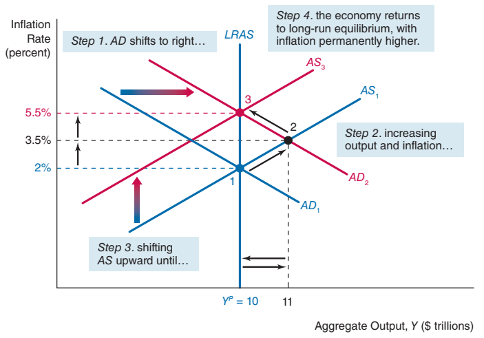
- Point 3 will be the new long-run equilibrium, if the central bank accepts that level of inflation.
- More on this next week.
- Next slide for details
Previous Slide’s Details: Read at Home
We start from the long-run equilibrium at point 1. The AD curve shifts to the right due to \(\uparrow \overline{A}\): we will have point 2.
At this point, \(Y>Y^P\) and inflation increases. The supply self-correction mechanism comes into work forcing the AS curve to shift until it passes to AS3 and GDP equals Potential GDP.
The short-run effect: an economic expansion and an increase in inflation.
The long run effect: inflation rises, but the economy returns to Potential GDP \(\left(Y^P\right)\).
For point 3 to be a long-run equilibrium, the central has to accept an inflation of 5.5% (much higher then 2%, the inflation that central banks like). Next week, we will see what happens if the central bank does not accept such inflation.
4. Aggregate Supply Shocks
A Temporary Negative Supply Shock
Suppose that oil prices increase temporarily \((\rho \uparrow)\).
. . .
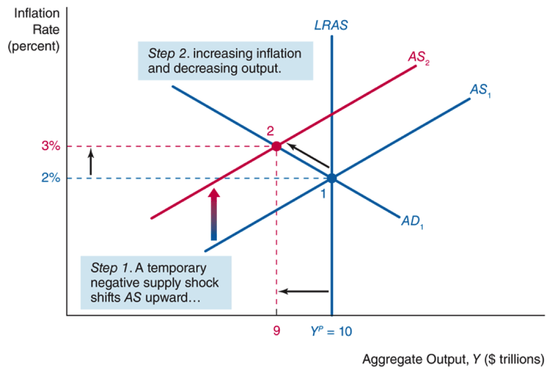
- A temporary supply shock has only temporary effects.
- But this also depends on the reaction of the central bank. More on this next week.
- Next slide for details
Previous Slide’s Details: Read at Home
We start from the long-run equilibrium at point 1. An increase in \(\rho\) shifts the AS curve to the left, from AS1 to AS2.
We move to point 2, where we have a higher inflation and also \(Y<Y^P\).
However, the productive capacity of the economy (the LRAS, also known as Potential GDP or \(Y^P\)) remains unchanged. So, at 2 we are in a recession
The self-correcting supply mechanism will make the adjustment along the AD1, back to the initial equilibrium point.
The short run effect: an economic recession and an increase in inflation.
In the long run: output and inflation return to their initial equilibrium, \(Y^P\) and \(\pi=2 \%\). But as we will see next week, this also depends on the reaction of the central bank.
A Permanent Negative Supply Shock
Suppose a permanent negative supply shock reduces Potential GDP: \(Y^P \downarrow\)
. . .
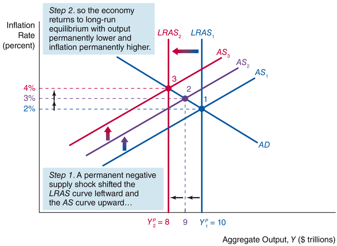
- A permanent supply shock has permanent effects.
- It \(\downarrow Y^P\) and \(\uparrow \pi\).
- But this depends also on the reaction of the central bank. More on this next week.
- Next slide for details
Previous Slide’s Details: Read at Home
We start from the long-run equilibrium at point 1. A permanent (negative) supply shock shifts supply to the left, from LRAS1 to LRAS2.
Inflation increases, shifting AS to the left, from AS1 to AS2, moving to point 2.
At this point we see \(Y>Y^P\), which causes inflation to increase again, shifting AS to AS3.
The new long-run equilibrium occurs at point 3.
The short-run effect: a fall in GDP and an increase in inflation.
In the long run: potential GDP falls and inflation rises, both on a permanent basis. However, this result also depends on the reaction of the central bank, as we will see next week.
5. Readings
Readings
Read Chapter 12 of the adopted textbook:
Frederic S. Mishkin (2015). Macroeconomics: Policy & Practice, Second Edition, Pearson Editors.