Fiscal Policy & the Government Budget

Week 11

Vivaldo Mendes

vivaldo.mendes@iscte-iul.pt

Instituto Universitário de Lisboa (ISCTE-IUL)

May 12, 2025

1. A Word of Caution

Most Controversial Issue in Macroeconomics

It is the ground where economics meets politics, at its best.
Fiscal policy involves:
- taxing/subsidizing people and corporations
- spending on goods and services
- hiring people for providing services to the community
It affects the distribution of income.
It affects the political landscape and the social equilibrium in a society.
What can be more controversial than this in a modern and open society?

Two Main Schools of Thought

Classicals. Main assumptions:
- Markets work very well.
- The best possible outcome is achieved with no government intervention.
- The government should provide only the goods&services associated with classical functions of the state: defense, justice, and order.
Keynesians. Main assumptions:
- Markets suffer from significant failures (market power, public goods, externalities, incomplete markets).
- The best possible outcome is achieved with government intervention.
- The government should provide the goods&services associated with the market failures, besides those associated with the classical functions of the state.
You. You should be aware of this dichotomy before making your opinion.

2. The Government Budget

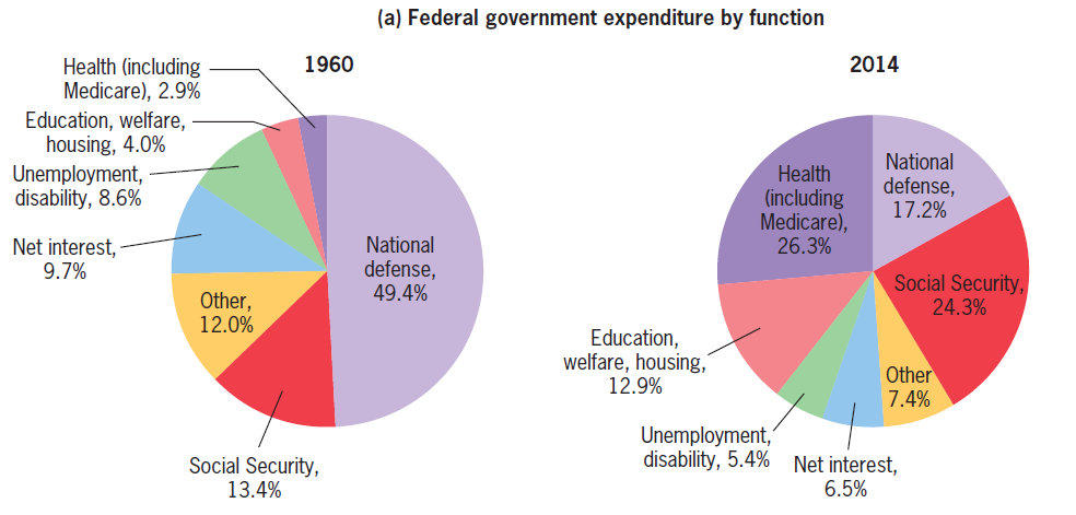
Federal Government Spending: 1960 vs 2014

From: Jonathan Gruber (2016). Public Finance and Public Policy, 5th Edition.

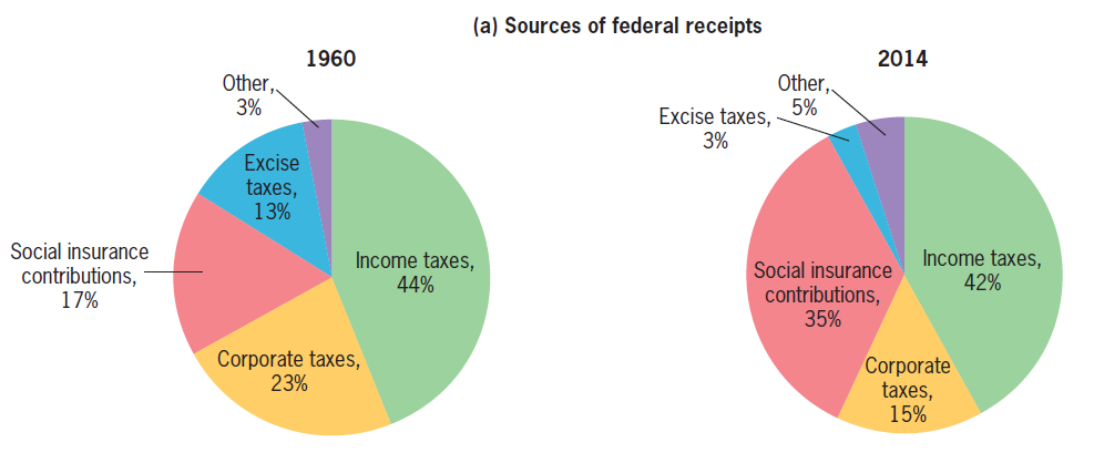
Federal Government Receipts: 1960 vs 2014

From: Jonathan Gruber (2016). Public Finance and Public Policy, 5th Edition.

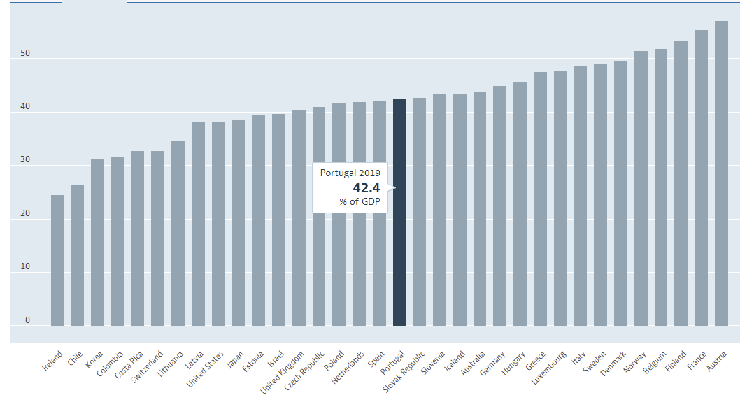
Public Spending as a % of GDP (OECD, 2019)

No, Portugal is not the country with the highest Debt/GDP ratio. OECD

3. The Size of Government Debt

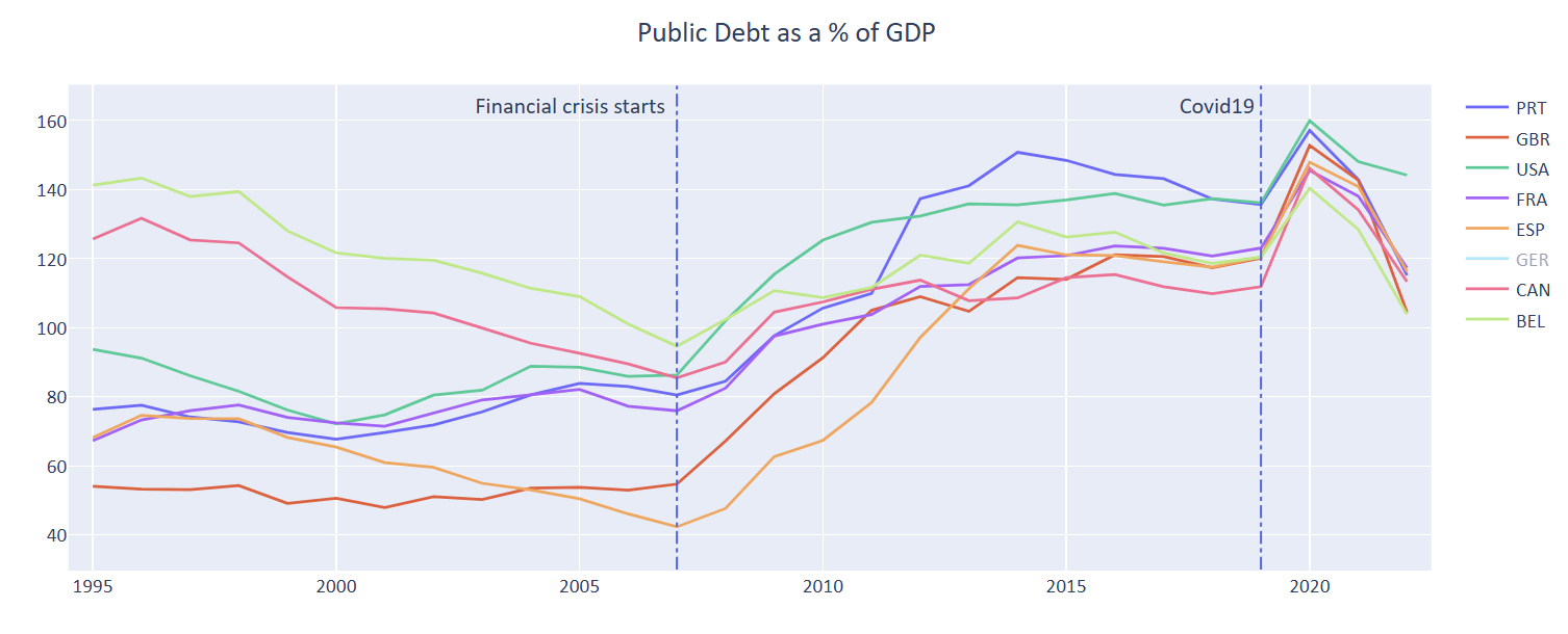
Public Debt as a % of GDP

Public debt/GDP ratio changes drastically with external shocks. From: OECD

USA: Federal Budget vs Federal Debt

A paradox: the US government run a deficit for decades, yet its debt/GDP ratio declined until 1981. From: FRED

Explaining the Paradox: the US Debt/GDP

The level of public debt as a % of GDP \(\left(d_t\right)\), is affected by three forces:

The primary deficit (deficit before interest payments) as a % of GDP ( \(p\) ).
The growth rate of real GDP \((g)\).
The real interest ratepaid on public debt \(\left(r_p\right)\). The equation that drives the evolution of public debt as a % of GDP is: \[ d_t=p+\left(\frac{1+r_p}{1+g}\right) d_{t-1} \tag{1} \]
If \(g>r_p\) , the level of \(d_t\) is sustainable.
If \(g<r_p\) , the level of \(d_t\) is unsustainable (it explodes over time).

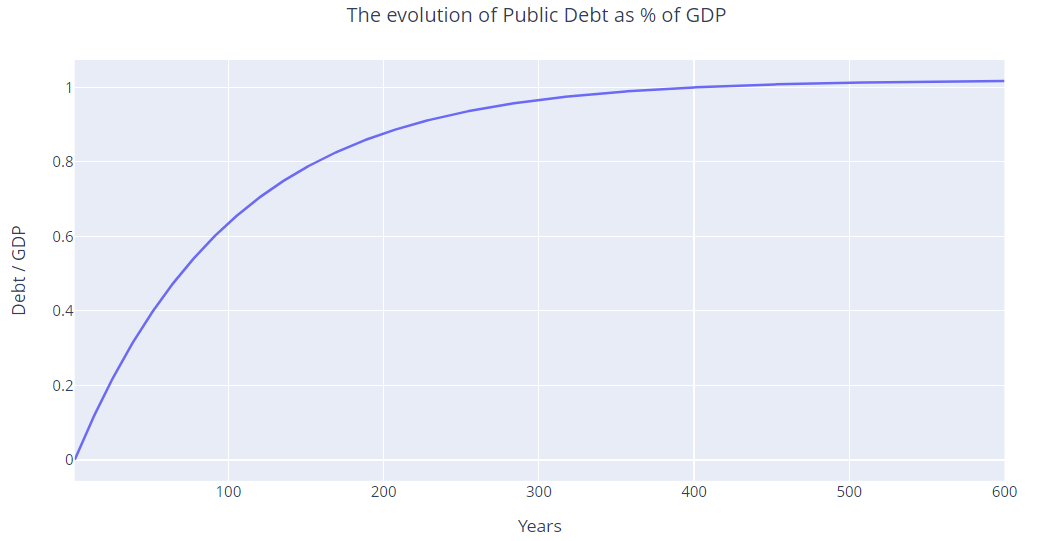
Public Debt Sustainability: An Exercise

Pessimistic scenario: \(p=0.1\%, g=2\%, r_p=1\%\). Surprise … the time span.

4. Aging, Taxation and the Size of Public Debt

The Shadows Behind Public Debt

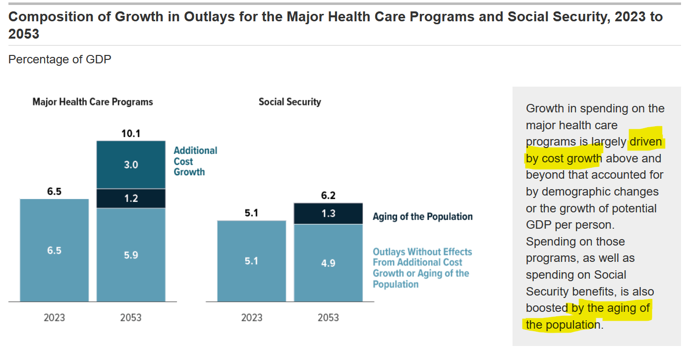
From: Congressional Budget Office: The 2023 Long-Term Budget Outlook

The “Problem”: the Aging of the Population

For the Congressional Budget Office aging is the major problem for public finances in the USA.

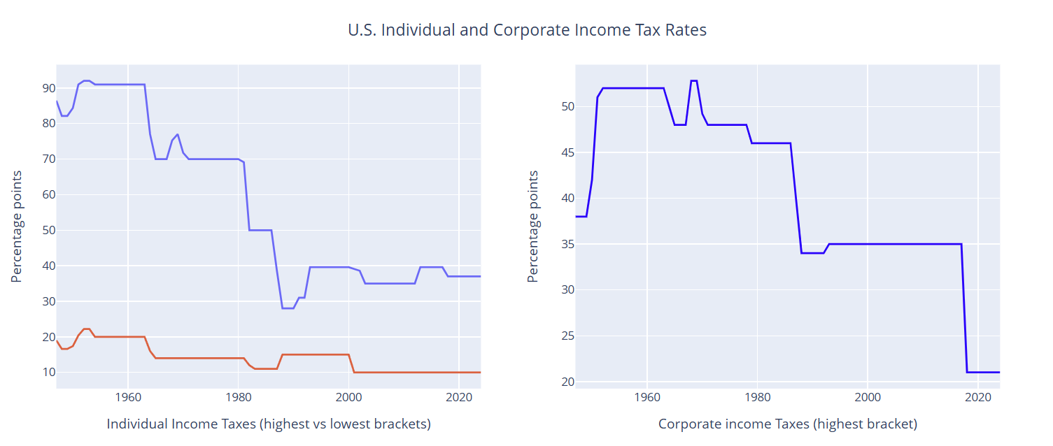
Another “Problem”: Income Taxation

Since the early 1960s, the highest tax brackets for individual and corporate income have dropped dramatically.

Two Fundamental Types of Public Spending

Public spending can be separated into two basic types:
- Mandatory spending
- Discretionary spending
Mandatory spending is the public spending that is difficult to reduce in a modern state: social security (pensions), medicare+medicaid (basic health care services), defense, justice, police, public schooling.
Discretionary spending can be increased or reduced to manage short-term business cycles : unemployment benefits, defense spending, investment subsidies, etc..

Discretionary Spending Has Come Down

From: US Congressional Budget Office Data

Mandatory Spending Has Not Skyrocket

From: US Congressional Budget Office Data

5. The Fiscal Multiplier

Why Using Fiscal Policy as a Policy Tool?

When the economy is hit by large negative shocks, the private sector (firms and households), if left alone, may not be able to stand up to the impacts of those shocks.
Examples: The Great Depression of the 1930s, the Great Recession of the 2000s, or the Covid19 pandemic.
Covid19: without the immediate help of governments (and central banks), our societies would be very different from what they still are.
In times of trouble: Households, small businesses, big corporations: “Please help!”

Why is Fiscal Policy Useful?

There are two fundamental reasons why active fiscal policy (increase spending/taxation) is used:

One reason is not economic, but rather social and political: to avoid serious social unrest. This is not the subject of our course.
The second reason is economic, the fiscal multiplier: \[ m^g=\frac{\Delta Y}{\Delta\overline{G}} \]
The fiscal multiplier says that if the government changes public spending \((\overline{G})\), it will change GDP \((Y)\).
The magnitude of the fiscal multiplier depends on the slope of the AS curve, as we will see.

The Fiscal Multiplier vs the Demand Multiplier

The demand multiplier (includes only the demand side): \(m\)
The fiscal multiplier (includes both sides: demand & supply): \[m^g= \frac{m}{1+ \varphi} \quad , \quad \varphi = m \phi \lambda \gamma\]
If \(\gamma =0\), they will equal because \(\varphi=0\).
When \(\gamma >0\), the fiscal multiplier will be lower than the demand multiplier.
The higher is \(\gamma\), the lower will the \(m^g\) be.
See next slides for the intuition.

Fiscal Multiplier: The Intuition

The higher is the AS’s slope, the lower will be the fiscal multiplier.

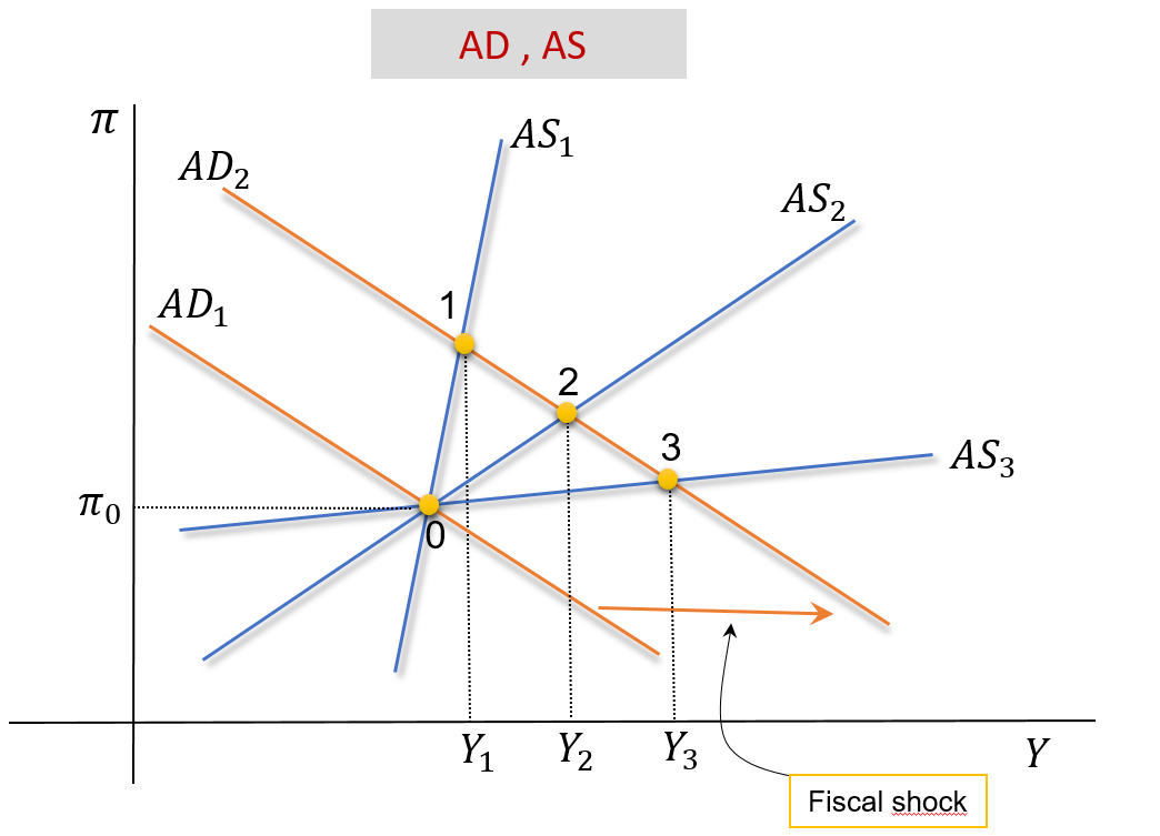
The same fiscal expansion will have a lower impact on \(Y\) if the AS is steeper.
\[\Delta Y_1 < \Delta Y_2 < \Delta Y_3\]
Higer slope of the AS: higher \(\gamma\)

Previous’s Slides Details: Read at Home

Suppose there is a positive shock on aggregate demand, such that AD1 moves to AD2.
The same shock will lead to different increases in GDP depending on the slope of the AS curve.
If the slope of the AS curve is very high (like AS1), the increase in GDP is tiny: from 0 to Y1.
If the slope AS is intermediate (like AS2), the increase in GDP is more significant than the previous case: from 0 to Y2.
If the slope AS is tiny (like AS3), the increase in GDP is considerable: from 0 to Y3.
The increase in GDP, caused by a shock in de AD, is maximal when the AS curve is horizontal; which occurs when \(\gamma=0\).

\(m^g\) proof: not compulsory reading

The AD curve: \(\quad Y=m \cdot \overline{A}-m \cdot \phi \cdot(\overline{r}+\lambda \pi)\)
The AS curve:\(\quad \pi=\underbrace{\pi^e}_{=\pi_{-1}}+\gamma\left(Y-Y^P\right)+\rho\)
Insert the AS into the AD, and solve for \(Y\):
\[Y = \frac{m}{1+\varphi}\overline{A} - \frac{m\phi}{1+\varphi}\overline{r} -\frac{m \phi \lambda}{1+\varphi}\pi^e + \frac{\varphi}{1+\varphi}Y^P - \frac{m \phi \lambda}{1+\varphi}\rho \tag{2}\]
To simplify things we defined:
- \(\varphi = m \phi \lambda \gamma\)
- \(\overline{A}=\overline{C}+\overline{I}-d \cdot \overline{f}+\overline{G}+\overline{N X}-c \cdot \overline{T}\)
Now, the fiscal multiplier can be easily seen in eq. (2): \[m^g=\frac{\Delta Y}{\Delta\overline{G}}=\frac{m}{1+\varphi}\]

6. Ricardian Equivalence

The Fiscal Multiplier: A Fallacy

In 1974, Robert Barro published a very famous paper.¹
Barro’s argument has become known as “Ricardian Equivalence” following an economist in the 19th century (David Ricardo)
He argued that, under certain conditions:
- Fiscal policy is totally irrelevant
- Fiscal policy produces no impact at all on economic activity and savings
Therefore, according to Barro, the previous theory (the fiscal multiplier) is a mere fallacy.

Certain Conditions Must Be Satisfied

The conditions that must hold for the Barro’s argument to be valid are:

Households must be homogeneous (all fully identicall)
Taxes can not be distortionary (no VAT taxes, no income taxes, and so on)
Generations must match (no old people, no young people)
Credit markets are perfect (no credit rationing)
People must have Rational Expectations (people make no forecasting errors about the future)

It is easy to see that none of these conditions are satisfied in the real world.

The Barro’s Argument

Suppose private agents are fully rational.
They react in a rational manner to any decision announced by the government to reduce taxes and compensate this reduction by issuing more public debt.
So private agents correctly forecast that, even though they may have to pay less taxes today, they will have to pay higher taxes in the future, so that the government can pay back its debt.
The net effect is zero: government spends more today, private agents save more today (to pay higher taxes in the future).
Aggregate demand and savings remain unchanged in the face of changes in fiscal policy.
In the end, nothing changes in real terms

7. Readings

Readings

Read Chapter 16 of the adopted textbook:

Frederic S. Mishkin (2015). Macroeconomics: Policy & Practice, Second Edition, Pearson Editors.