Macroeconomic Policy & Extreme Shocks
Week 10
1. Fed’s Dual Mandate (Again)
The Fed’s Dual Mandate
The Fed’s dual mandate according to the Federal Reserve Bank of Chicago
. . .
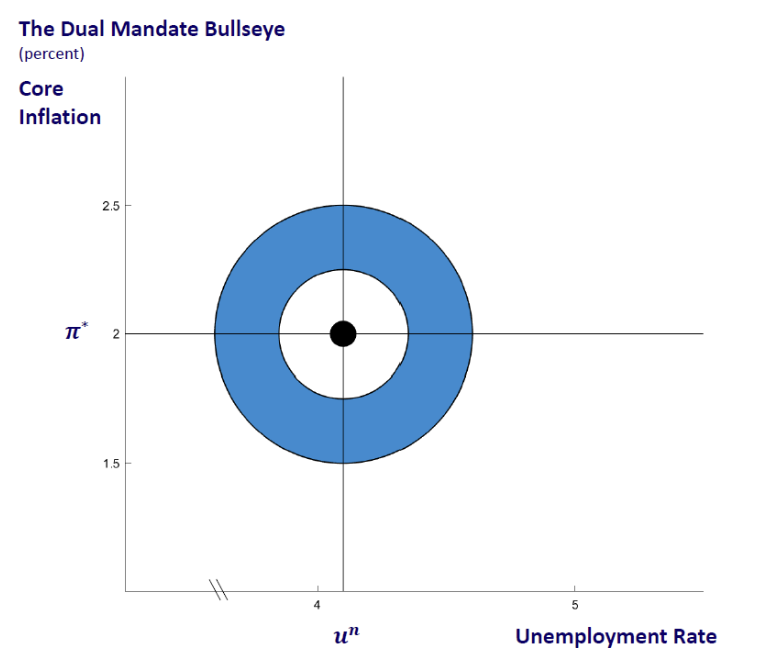
The FRB of Chicago calls the target inflation rate by \(\pi^*\)
We call it \(\pi^{_T}\)
The meaning is the same
2. Inflation Targeting
Inflation Rate Target
All central banks in advanced countries have an optimal value for inflation they want to achieve. This is called the inflation target:\[\color{blue}{\pi^{_T}}\]
. . .
\(~~~~~~~~~~~~~~~~~~~~~\)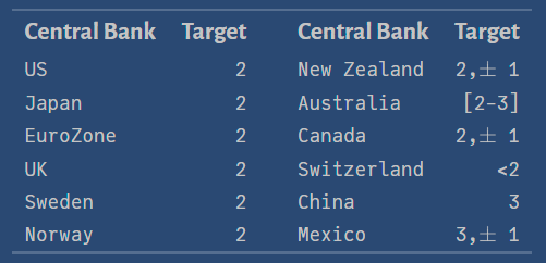
Source: Central Bank News
Targeting Inflation: Two Ways to Do It
There are two different ways of looking at the target value:
- \(\pi^{_T}\) is a ceiling. The central bank suffers a loss if \(\pi>\pi^{_T}\)
- \(\pi^{_T}\) as a true target . The central bank suffers a loss if \(\pi \neq \pi^{_T}\).
Examples:
- Ceiling: Switzerland (still now), ECB (until July 2021)
- True Target: all central banks in advanced economies
What’s The Problem With \(\pi^{_T}\) as a Ceiling?
- If \(\pi^{_T}\) is used as a ceiling, central banks will be biased to keep inflation systematically below the target.
- It may lead to “too low inflation” or even deflation
- The costs to the society will be higher than if the target were reached
- ECB changed its monetary policy strategy in July 2021 for that reason:
European Central Bank, 8 July 2021:
“The Governing Council considers that price stability is best maintained by aiming for a 2% inflation target over the medium term. This target is symmetric, meaning negative and positive deviations of inflation from the target are equally undesirable.”
3. Monetary Policy Rules
What is a Monetary Policy Rule?
- Central banks have to react to the events in the economy.
- But what macroeconomic variables should they use to guide their decisions?
- The Monetary Policy Rule provides the answer to this problem.
- We have already studied a simple version of such a rule in previous weeks:
- The MP curve (we can call it now as the Textbook Rule)
- We are going to discuss a new rule in the next slides:
- The Taylor Rule (proposed by John Taylor in 1993).
The Textbook Rule (the MP curve)
How the textbook rule performs, compared with the Fed Funds Rate?
We may recall our well-known MP curve (rule) and the Fisher equation: \[ r=\bar{r}+\lambda \cdot \pi \tag{MP curve} \] \[ i=\pi+r \tag{Fisher eq.} \]
Insert the MP in the Fisher eq., and the Fed funds rate \((i)\) comes out as: \[ i=\bar{r}+\pi+\lambda \cdot \pi \]
Using data on \(\overline{r}, \pi, \lambda\), we can calculate \(i\) from this rule.
Then, we can compare this \(i\) with the Fed Funds Rate that the Fed sets over time.
See the following figure.
The Textbook Rule vs the Fed Funds Rate
We set: \(\lambda=0.5, \overline{r}=2\). The textbook rule performs very badly.

Policy Rules & How Policymakers Use Them
- The MP rule studied in previous weeks was helpful in explaining the basic concepts in macroeconomics.
- However, in reality, central banks use a more sophisticated rule for making decisions about \((i)\).
- The other items always included in the rule are:
- The target inflation rate
- The output-gap
- A trending factor to incorporate prudence (not covered here)
- Check the different rules used by the Fed here: Policy Rules and How Policymakers Use Them
The Taylor Rule Elements
The Taylor Rule
- The Taylor Rule indicates what is the level of the nominal interest rate that the Fed should set:
\[i = \bar{r} + \pi + \lambda_{\pi} \cdot {\color{blue}\pi^{gap}} + \lambda_{_{Y}} \cdot {\color{red}Y^{gap}}\]
- Where \(\lambda_{\pi}\) and \(\lambda_{_{Y}}\) are parameters
- Taylor proposes the following values for the exogenous variables and parameters: \[ \overline{r}=2 \% \ \ , \ \pi^{_T} =2 \ , \ \lambda_{\pi}=\lambda_{_{Y}}=0.5 \]
- Let’s see how the Taylor Rule performs when compared with the Fed Funds Rate.
The Taylor Rule vs the Fed Funds Rate
Weights: 0.5 for the output-gap, 0.5 for the inflation-gap.

The New Taylor Rule vs the Fed Funds Rate
Weights: 1.0 for the output-gap, 0.5 for the inflation-gap: it performs better

Taylor Rule on Autopilot?
Why hasn’t the Fed put the federal funds rate on a Taylor rule autopilot ?
- Recall the logic behind rules in monetary policy:
- No rules leave room for speculation, higher uncertainty, and risk.
- Too strict rules leave room for too much punishment.
- Best approach: use a rule … with wisdom, with some flexibility.
- The Taylor Rule may be pretty helpful in “normal” situations.
- But terrible shocks have hit Western economies:
- Great Recession in 2008-2011
- COVID pandemic in 2020-21
- Galloping oil prices
- The war in Ukraine, and now a war in the Middle East (Iran).
- So, exceptional circumstances can only be dealt with exceptional measures.
4. Strange Times:
– From the Fear of Deflation to Galloping Inflation –
Living Through Strange Times
Since the early 2000s, Western economies have been hit by a succession of terrible shocks (see previous slide)
- Some have a political nature
- Some have a financial nature
- Some have a health nature
Those shocks have led to two extreme situations:
- Explosive inflation: from mid 2021 to mid 2023
- Fear of deflation: from 2008 up to 2021
Explosive Inflation
- In Western countries, inflation reached very high levels … very fast

How to Deal With Explosive Inflation?
In the summer of 2022, it was very “fashionable” to argue that the only way to control explosive inflation was to cause a severe recession.
For example, a very influential economist, Larry Summers, defended that:
“We need five years of unemployment above 5% to contain inflation – in other words, we need two years of 7.5% unemployment or five years of 6% unemployment or one year of 10% unemployment.” speech in London, 20 June 2022. Bloomberg
Summers was not alone: there was quite a large chorus on this camp.
Fortunately, their predictions proved wrong: inflation has been coming down and unemployment has not gone up!
The Fear of Deflation
- 20 years ago, it was inconceivable to think that nominal interest rates could be \(0 \%\) or even negative.
- That world collapsed in the Great Recession of 2008-2011 and subsequent developments.
- Two major types of responses by central banks:
The Fear of Deflation
- 20 years ago, it was inconceivable to think that nominal interest rates could be \(0 \%\) or even negative.
- That world collapsed in the Great Recession of 2008-2011 and subsequent developments.
- Two major types of responses by central banks:
- Many countries:
- Negative nominal interest rates if necessary
- For example, in the summer of 2021 they were negative in Switzerland, Euro Zone, Japan, Denmark, Sweden, and others.
- In the US:
- Cut nominal interest rates as much as possible, but stopped at the \(0 \%\) limit.
- Not going below \(0 \%\), is what we mean by the Zero Lower Bound on \((i)\).
Switzerland: Pinnacle of Financial Stability
. . .
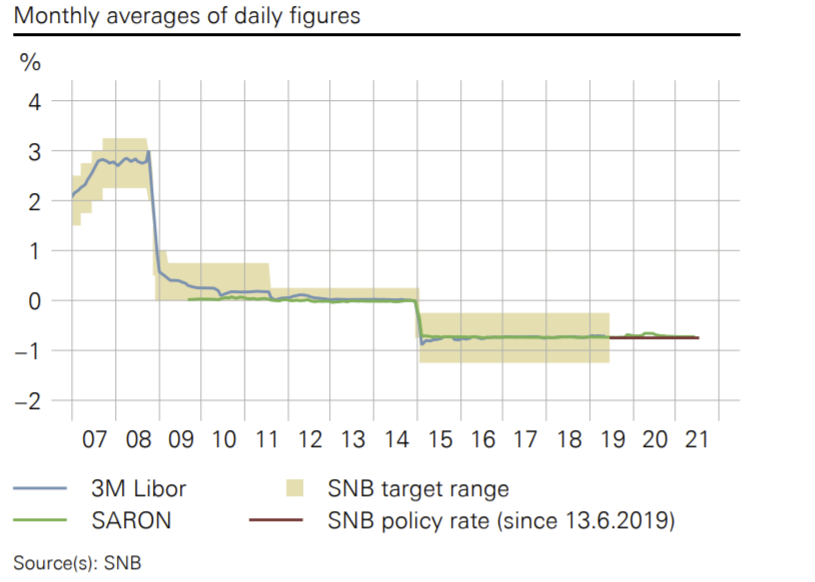
- The Swiss National Bank (SNB) kept the interest rate at \(-0.75 \%\) for a long time.
- In September 2022, the SNB decided to raise the rate to \(+0.5 \%\).
EURIBOR: The Unthinkable
. . .
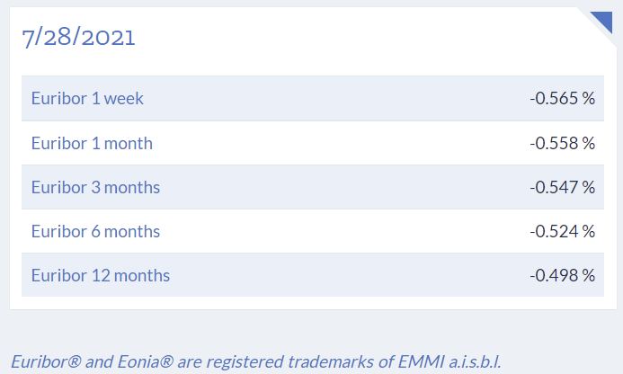
- Euribor rates were negative (for all maturities) in the summer of 2021.
- Currently, they range from \(1.9\%\) and \(2.4\%\)
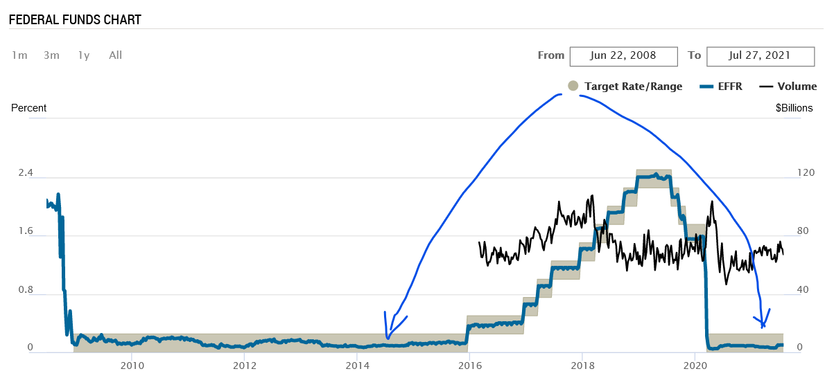
The ZLB: the US case
The Fed Funds Rate is the blue line (it is the overnight market rate); the FED sets the range (the gray interval) in the lower limit (0%). FRB of New York
ZLB: Consequences
- Until the ZLB is reached, the MP and AD curves have their normal representations.
- However, when the ZLB is reached, there will be a kink in those two curves, and their slopes become the opposite of what they were.
- This has dramatic consequences for:
- The macroeconomic equilibrium
- GDP, inflation and unemployment
- The way monetary policy is conducted
- The way fiscal policy is used as a policy tool
ZLB: Representation of the MP curve
. . .
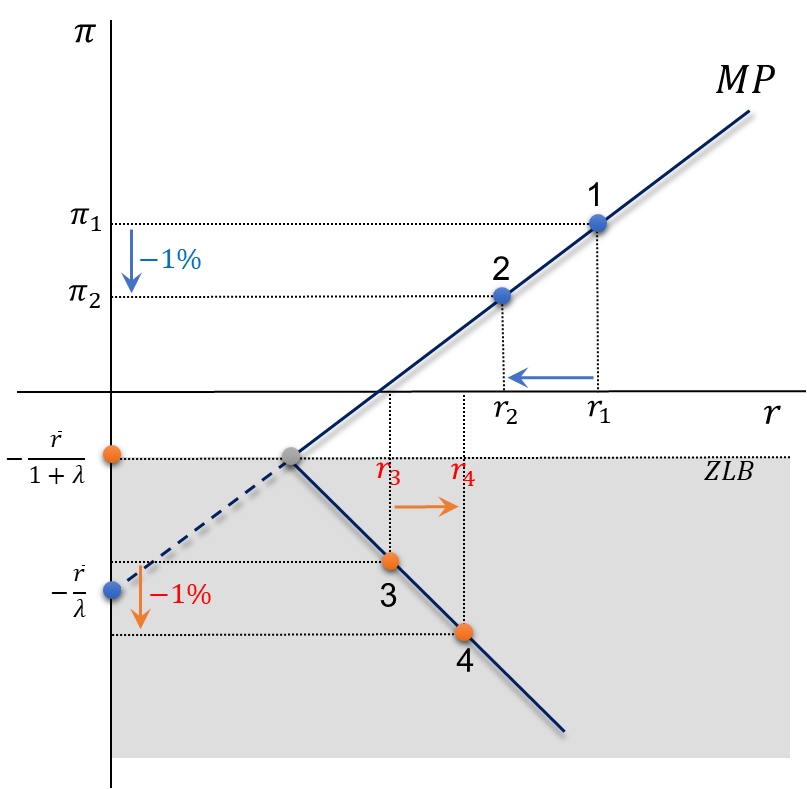
- MP in the normal zone: \[r=\overline{r}- \lambda \pi\]
- MP in the ZLB: \[r=-\pi_{_{ZL}}\]
ZLB: Representation of the AD curve
. . .
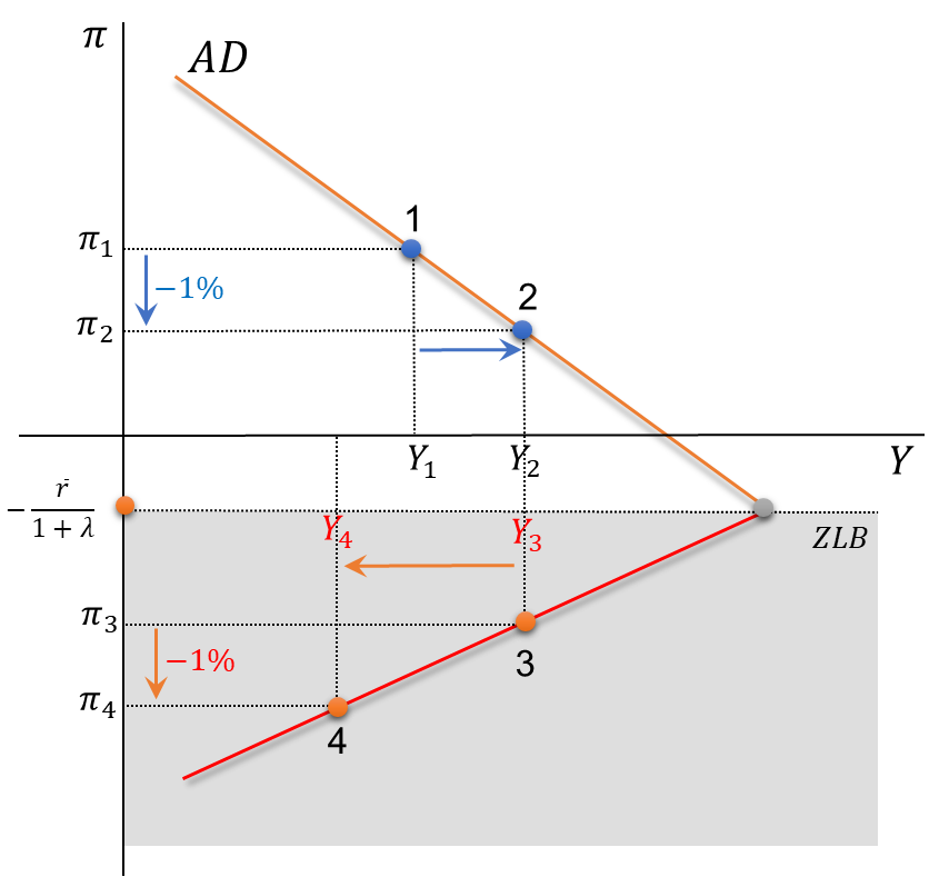
- AD in the normal zone: \[Y=m \cdot \overline{A}-m \cdot \phi \cdot(\overline{r}+\lambda \pi)\]
- AD in the ZLB: \[Y=m \cdot \overline {A}+m \cdot \phi \cdot \pi_{_{Z L}}\]
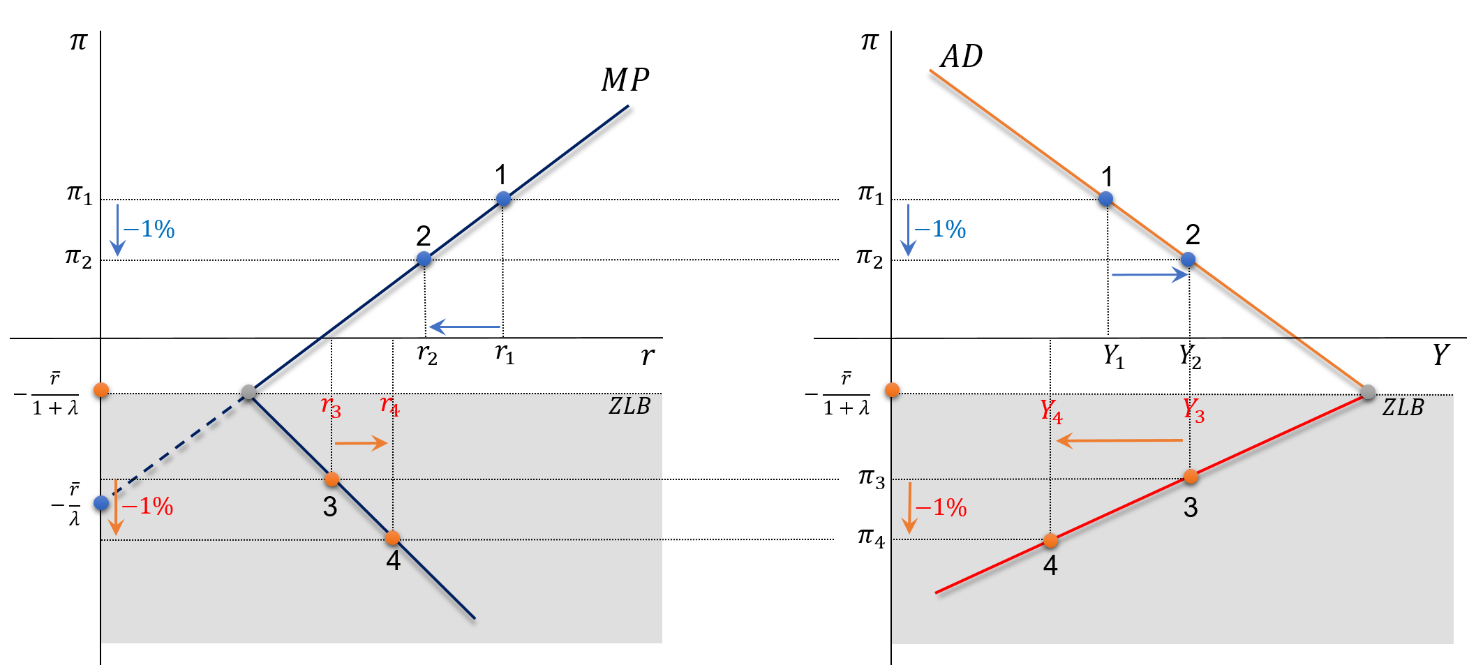
ZLB: Representation of AD and MP Curves
A reduction in inflation of \(1 \%\) causes different (opposite) impacts upon \(Y\) and \(r\) when comparing the ZLB with the normal zone.
5. Strange Things Happen in the ZLB
Not covered in this course.
Alice Trough the Looking Glass
Paul Krugman, Nobel Prize winner 2008: the ZLB is a “Alice through the looking glass” experience.
Strange Things I: Deflation Trap
Suppose the economy falls into the ZLB (point \(1_{Z L}\) ). It will end up in the long-term equilibrium \(2_{Z L}\) and remain trapped there forever.

Previous Slide’s Details: Read at Home
Consider that, for some reason, the economy is operating at point \(1_{Z L}\) in the ZLB. This point is determined by the intersection of the AD curve (which in the ZLB we call by ADzl) and the initial AS curve (AS1).
At point \(1_{_{Z L}}\), the economy has negative inflation \((\pi=-3.6 \%, Y=13.4)\), \(Y^P=14\) trillion dollars. This point represents a short-run equilibrium but not a long-run one because we are in a recession.
In a recession, inflation is forced to come down, which will shift the AS to the right (AS1->AS2). This movement will only stop when the recession is eliminated by declining inflation, which occurs when the AS2 crosses the ADzl at point \(2_{Z L}\).
Point \(2_{_{Z L}}\) represents the long-term equilibrium for this economy, with \((\pi=-2 \%)\), and \(Y=Y^P=14\). The economy will be stuck at this equilibrium forever until some new major shock forces it to move away from such a trap.
This case looks like what has happened to Japan since the late 1990s.
Strange Things II: Secular Stagnation
Suppose a big negative demand shock forces the economy to move to point 2. In the long term, it will end up at point 3.

Previous Slide’s Details: Read at Home
Consider the economy is operating at point 1, with inflation of \(\pi_1=2 \%\) and \(Y=Y^P=14\) trillion dollars: it is a long-run equilibrium.
Suppose that the AD suffers a huge negative shock and the economy moves to point 2. This point is not a long-run equilibrium because we are in a large recession.
In a recession, inflation decreases, and the AS shifts to the right. The economy moves to point 3.
At point 3, demand is insufficient to match supply at a higher GDP level. So GDP is stuck at a level that is permanently lower than what the economy can produce ( \(Y^P=14\) ). Only very aggressive monetary and fiscal expansionary policies can (by forcing a large increase in AD ) remove the economy from such stagnation.