
Week 10 - Macroeconomic Policy and Extreme Shocks
Exercises
Macroeconomics, ISCTE-IUL
Vivaldo Mendes, Ricardo Gouveia-Mendes, Luís Clemente-Casinhas
May 2005
Packages used in this notebook
Exercise 1. The Fed's Dual Mandate (again)
One of the Fed branches—the Federal Reserve Bank of Chicago—published an image that explains the Fed's double mandate in a very simple way. The figure can be found below, taken from here.
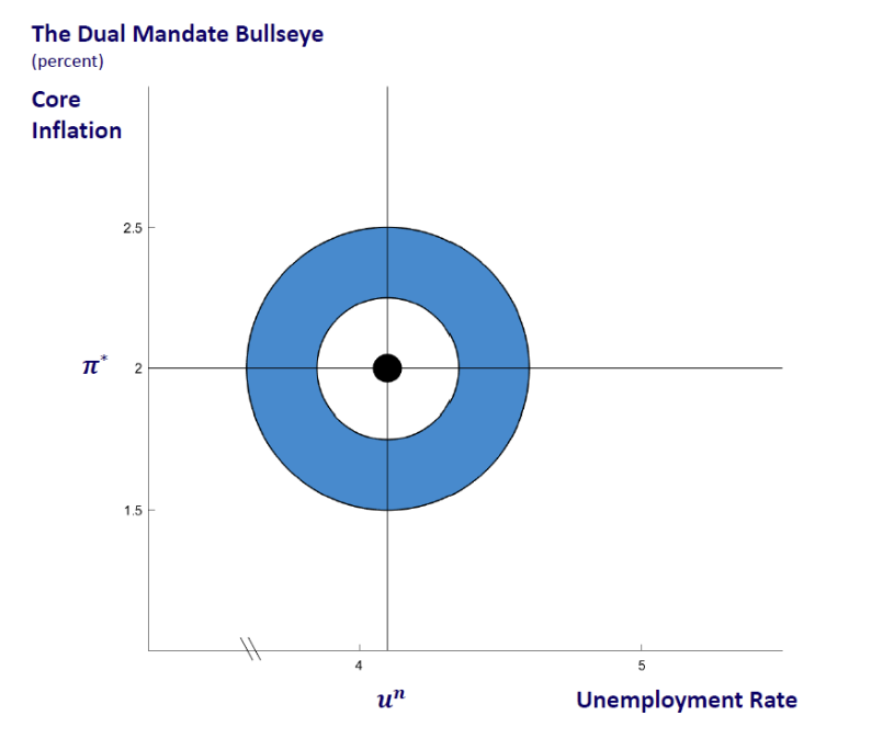
👉 a) In your own words, what are the two fundamental goals of the Fed over time?
Answer (a)
The two fundamental goals of the Fed over time are:
👉 b) Given what you have studied in this course, suppose the natural unemployment
Answer (b)
As
👉 c) Given what you have studied in this course, suppose the rate of inflation
Answer (c)
As
👉 d) Suppose that the two cases above co-exist simultaneously. What should the Fed do in this case? Give up one of them, give up both, or balance both in some way?
Answer (d)
If the two cases co-occur, the Fed should balance the two goals over time. In the past, the Fed has usually given higher priority to controlling inflation than to reducing unemployment. Still, that decision is totally dependent on the composition of the Fed's board at each particular period.
Exercise 2. Unemployment and recessions
The following figure presents the evolution of the unemployment rate (UR) and the Fed Funds Rate (FFR) for the US economy from the mid 1960s to 2024.
👉 a) What happens to the unemployment rate in every single recession in this period? Why?
Answer (a)
In all recessions, the unemployment rate increases significantly.
Why? Because a recession is defined as a substantial reduction in GDP below Potential GDP, which leads to a significant decrease in employment and a consequent increase in the unemployment rate.
👉 b) What happens to the Fed Funds Rate in every single recession in this period? Why?
Answer (b)
In all recessions, the Fed Funds Rate decreases significantly.
Why? A recession leads to a substantial increase in the unemployment rate, and one of the Fed's main goals is to "support maximum employment". Therefore, the Fed has to reduce interest rates to stimulate demand, which in turn will increase GDP and employment.
👉 c) The following figure presents a cross-plot between the US's unemployment and Fed Funds rates between 1955 and 2024, and the correlation coefficient between these two variables is close to zero
Answer (c)
The correct remark is (iii).
👉 d) Are there other major macroeconomic variables that directly affect the decision of the Fed regarding the FFR? If yes, what are they?
Note
The main reason macroeconomic theory is helpful is that it prevents us from making stupid mistakes that are masked as irrefutable observations. It is easy to see that in the plot above, there is no significant correlation between these two macroeconomic aggregates. Therefore, we would be inclined to prematurely conclude that the Fed does not react to unemployment. Why is this speedy reasoning incorrect?
Answer (d)
As the Fed has a "dual mandate" with the goals of maximum employment and stable prices, the other major macroeconomic variable affecting the Fed's decisions regarding the FFR is the inflation rate. That is why we do not see a clear causality between the FFR and the unemployment rate in the plot above, as there is another major player in this game, which is not present in that figure.
Exercise 3. Inflation targeting
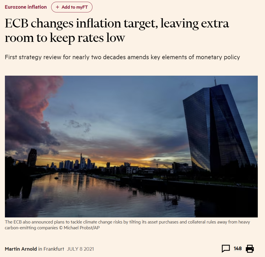
On 8 July 2021, the European Central Bank (ECB) announced a revision of its monetary policy strategy for the first time since its creation in 1998. From the article above in the Financial Times, one can read:
"The central bank said its new target of 2 per cent was symmetric, “meaning negative and positive deviations of inflation from the target are equally undesirable”. The new target is a medium-term objective with flexibility to fluctuate in either direction in the short term [and] said it could tolerate temporary moves beyond that point, in a shift that gives policymakers flexibility to keep interest rates at historic lows for longer”.
👉 a) Figure 1 plots the data about inflation in the EuroZone (EZ) and Portugal since 1998. Why do you think the ECB stresses "the symmetric deviations of inflation from the target"?
Answer (a)
The ECB stresses "the symmetric deviations of inflation from the target" to clarify that it will not tolerate inflation rates below 2%, no matter how low and stable they may be. Inflation above target and below target should be treated similarly.
👉 b) Why do you think the article stresses "...in a shift that gives policymakers flexibility to keep interest rates at historic lows for longer”?
Answer (b)
Usually, using the target as a "ceiling" leads to a situation where inflation is too low. In the summer of 2021, the ECB feared deflation and wanted to increase inflation to the 2% target level. Changing the strategy to "symmetric deviations" would lead to higher inflation, requiring keeping interest rates very low for an extended period.
👉 c) Figure 2 below shows the inflation deviations from its target, according to the old strategy (we will call it "Loss1"), while Figure 3 displays the deviations according to the new strategy ("Loss2").
Note
If central banks do not achieve the 2% target level for inflation, they do their job poorly. They will be penalized sooner or later because the economy (and society) suffers a Loss of welfare from those deviations. The greater the deviations, the greater will be Loss society will bear.
| Loss to society | mean | min | median | max | standard dev. | |||||
|---|---|---|---|---|---|---|---|---|---|---|
| Euro Zone (Ceiling) | 0.1799 | 0.0 | 0.0 | 2.1 | 0.3579 | |||||
| Euro Zone (True target) | 0.7568 | 0.0 | 0.6 | 2.6 | 0.6422 | |||||
| Portugal (Ceiling) | 0.5081 | 0.0 | 0.0 | 3.1 | 0.7180 | |||||
| Portugal (True target) | 1.2081 | 0.0 | 1.2 | 3.8 | 0.8148 |
Answer (c)
In the previous figure, we can easily observe why the central bank's loss function is dramatically affected by having only positive deviations from the target as its argument or by having both positive and negative deviations as arguments. The first case can be written in the following way:
while the second case has to be written using the absolute value operator:
The left-hand panel (Fig. 2) shows the first case. The right-hand side panel (Fig. 3) shows the second case; the losses are significantly much more significant than those in the left panel. This fact is the fundamental reason the ECB has decided to produce a drastic reform in its monetary policy strategy after more than twenty years since it started to operate.
The means of the Loss function according to each rule (the old strategy, which considered only positive deviations from the target, and the new strategy, which includes both positive and negative deviations) are presented in the following table.
👉 d) If you had responsibilities as a watchdog of the European Central Bank (for example, as a member of the European Parliament), and the ECB President argued that they had been doing a good job because the Loss to society was very small according to the old strategy, what would your position be?
Answer (d)
I would say that the ECB President was trying to mislead the public because Figure 3, not Figure 2, gives the true cost (loss) to society. In the case of the Eurozone as a whole, the actual Loss (Figure 3) is 4.2 times higher than the Loss presented by the old strategy in Figure 2 (0.757/0.18=4.2), and I would argue that the ECB had to change its approach by considering symmetric deviations instead of positive deviations only.
Exercise 4. The Textbook Rule (MP curve)
In week 5 we introduced the MP curve into our framework:
where
where
Interestingly, we can easily check whether a central bank (like the Fed) followed such a rule (MP curve) to set its nominal interest rates. We can collect data on
| Quarters | PotGDP | GDP | CPI | FFR | |||
|---|---|---|---|---|---|---|---|
| Date | Float64 | Float64 | Float64 | Float64 | |||
| 1 | 1960-01-01 | 3491.81 | 3517.18 | 1.4 | 3.93 | ||
| 2 | 1960-04-01 | 3527.85 | 3498.25 | 1.8 | 3.7 | ||
| 3 | 1960-07-01 | 3563.32 | 3515.39 | 1.4 | 2.94 | ||
| 4 | 1960-10-01 | 3597.51 | 3470.28 | 1.4 | 2.3 | ||
| 5 | 1961-01-01 | 3631.1 | 3493.7 | 1.5 | 2.0 | ||
| 6 | 1961-04-01 | 3662.76 | 3553.02 | 0.9 | 1.73 | ||
| 7 | 1961-07-01 | 3695.59 | 3621.25 | 1.2 | 1.68 | ||
| 8 | 1961-10-01 | 3729.38 | 3692.29 | 0.7 | 2.4 | ||
| 9 | 1962-01-01 | 3765.8 | 3758.15 | 0.9 | 2.46 | ||
| 10 | 1962-04-01 | 3805.31 | 3792.15 | 1.3 | 2.61 | ||
| 259 | 2024-07-01 | 22800.6 | 23386.2 | 2.6 | 5.26 | ||
👉 a) In the figures below, we plot the Federal Funds Rate (the FFR, our
Answer (a)
No, it does not. The gaps between what the textbook rule predicts and what the Fed has done (FFR) are huge, sometimes on the verge of 10 or even 15 percentage points.
👉 b) Given what we discussed in Exercise 1, in your opinion, why does the textbook rule perform so poorly in the case of the Fed?
Answer (b)
It performs exceptionally poorly because the Fed sets nominal interest rates considering the natural real interest rate and the inflation rate (as the textbook does), but it also takes into account what happens to unemployment (which is not included in the textbook rule for simplicity).
Exercise 5. The Taylor rule
In 1993, John Taylor from Stanford University presented a monetary policy rule that became very famous. He conjectured that the Fed, according to its dual mandate, should set nominal interest rates according to the equation:
where
We will apply the same procedure as in the previous exercise. Let us insert the data into the notebook:
👉 a) In the figure below, we compare what the Taylor Rule predicts against the nominal interest rate that the Fed actually sets (the FFR). Does this rule better explain the Fed's decisions concerning the Fed Funds Rate than the textbook rule?
Answer (a)
The deviations of the FFR from the values given by the Taylor rule are much smaller than in the previous rule (the textbook rule). Therefore, the Taylor rule performs better than the previous one.
👉 b) Can you provide evidence that having a Taylor Rule in autopilot may lead to extreme "punishments" for the economy? Examples where applying this rule would lead to unbearable economic situations.
Answer (b)
There have been several periods when the Fed Funds Rate (FFR) was systematically much lower (or much higher) than the value given by the Taylor rule. We provide some examples that look awkward from an economic point of view:
In the early 1980s, the Taylor rule suggests that the Fed should have had interest rates much lower than it did. For example, in July 1983, the FFR was 7.14 percentage points higher than as indicated by the Taylor rule.
In July 2009, at the center of the Great Recession, while the Fed reduced the FFR to zero, the Taylor rule indicates that the Fed should have reduced those rates to
Another awkward example is what the Taylor rule suggests the Fed should have done recently. In April 2022, the Fed had the FFR at
Exercise 6. A Good Rule: the "First-Difference" rule
The Taylor rule is one of the rules the Fed uses when deciding to change (or maintain) nominal interest rates, and, as we saw in the previous exercise, it does not perform very well. That is why the Fed uses also other rules. In this website Policy Rules and How Policymakers Use Them, the Fed describes five different rules that it usually takes into consideration in its decision-making process. One of them is called "The First-Difference" rule and is expressed as follows:
where
👉 a) In the figure below, we plot the First-Difference rule and the actual Fed Funds Rate. Considering the gaps between what the rule predicts and the actual Fed Funds Rate, does this new rule perform better or worse than the Taylor rule seen in the previous exercise?
Answer (a)
The First-Difference rule performs much better than the Taylor rule, for two reasons: (i) the gaps between what the rule predicts and the actual Fed Funds Rate are much smaller than in the case of the Taylor rule, and (ii) the First-Difference rule does not lead to extremely abnormal outcomes like the Taylor rule does (e.g., –3% in April 2020, and +13.4% in April 2022).
👉 b) What happens when extreme events knock-on economic activity when compared to the Taylor rule? For example, what happened during the Great Recession of 2008-2010, the Covid pandemic in 2020, or the recent rampant inflation in 2022/2023?
Answer (b)
When the economy faces extreme events like those mentioned in the question above, this rule avoids the dramatic changes in the Fed Funds Rate as those that arise from the Taylor rule. For example, consider what happened in July 2009 (in the middle of the Great Recession): the Taylor rule indicated that the Fed should have reduced the Fed Funds Rate to
👉 c) Given the evidence in the three rules that we have been discussing, are monetary policy rules useless?
Answer (c)
Bad rules are useless, but good rules are beneficial because if the central bank follows good rules when conducting monetary policy, there will be less uncertainty in the economy. This less uncertainty arises because private agents know that the central bank has a rule, a sound/credible rule, has a commitment to follow such rule, and they will react to the shocks that hit the economy in accordance with the behavior of the central bank. Private agents know what to expect from the central bank, and this reduces uncertainty.
Exercise 7. The Volcker Disinflation, 1980–1986
On page 309 in the textbook:
"When Paul Volcker became the chairman of the Federal Reserve in August 1979, inflation had spun out of control, and the inflation rate exceeded 10%. Volcker was determined to get inflation down. By early 1981, the Federal Reserve had raised the federal funds rate to over 20%, which led to a sharp increase in real interest rates. Volcker successfully brought inflation down, with the inflation rate falling from 13.5% in 1980 to 1.9% in 1986. The decline in inflation came at a high cost: the economy experienced the worst recession up to that time since World War II, with the unemployment rate soaring to 9.7% in 1982."
In the two figures below, we provide further context for this period by providing evidence about the inflation rate (we use headline inflation in this exercise), the Fed Funds Rate (FFR), and the growth rate of international oil prices.
👉 (a) What was the Volcker disinflation?
Answer (a)
Volcker disinflation occurred during the 1980s, a period of unprecedentedly high inflation in the US and all Western economies. The Fed conducted a highly aggressive monetary policy, leading to an abrupt and brutal increase in real interest rates to reduce high inflation figures.
👉 (b) By inspecting the two figures above, which cover the period of the Volcker disinflation, how does the behavior of the Fed Funds Rate and international oil prices affect the US economy?
Answer (b)
The real interest rate (FFR minus Inflation) increased dramatically in the 1980s compared to previous decades. For example, in June 1981, it was higher than 9% (19.1%-9.7%=9.4%). These huge real interest rates led to a massive decline in aggregate demand in the US economy, which was expected to lower inflation.
The price of oil in international markets suffered a monumental decline throughout the 1980s. Notice that the annual growth rate of oil prices in April 1980 reached an astronomical figure of
👉 (c) Can we explain that sharp decline in inflation in the 1980s using our AD/AS/MP model?**
Answer (c)
Yes, the AD/AS/MP framework can easily explain what happened to inflation in the US during the 1980s. This is why models are helpful.
The Fed aggressively increased interest rates in the early 1980s. This increase shifted the MP curve to the left, leading to higher real interest rates for every level of inflation.
In our model above, the shift in the MP curve forces the AD curve to move to the left, creating a recession and lower inflation. The economy will gradually recover, and the recession will gradually vanish while inflation comes down step by step.
The process in (1) and (2) will significantly speed up if oil prices come down year after year, as they did in the 1980s. If oil prices go down, the AS curve will shift down (to the right), reducing inflation further and leading to higher GDP.
At the end of this process, we have lower inflation and no recession. The economy had to pay a high price for reducing inflation from
Exercise 8. Inflation and the Scariest Opinion of 2022
In the Wall Street Journal, Sept. 7, 2022, Jason Furman – a Professor at Harvard University and a former Chair of the Council of Economic Advisers of President Barack Obama – published an Op-Ed. that ran with the title "Inflation and the Scariest Economics Paper of 2022". The scariest paper can be found here and was written by two IMF economists and Larry Ball from John Hopkins University. The principal message from this paper was:
"To bring price increases down to 2%, we may need to tolerate unemployment of 6.5% for two years."
Earlier, on June 20 of the same year, another highly respected economist, Larry Summers, made the same point even more forcefully in a speech in London:
"We need five years of unemployment above 5% to contain inflation – in other words, we need two years of 7.5% unemployment, or five years of 6% unemployment, or one year of 10% unemployment." Bloomberg
Considering the evolution of inflation (CPI), unemployment (UR), and oil prices (Oil) in the US economy that is depicted in the figure below, answer the following questions:
👉 a) why do you think economists and policymakers were so worried about inflation in the middle of 2022?
Answer (a)
In the summer of 2022, US inflation reached close to 9%, the highest level since 1980.
Economists and policymakers feared that the Fed would be unable to contain inflation. If inflation continued to increase even further, people would start to doubt whether the Fed would be able to control inflation, high inflationary expectations would set in, and the situation in the late 1970s would come back to haunt us with unmanageable inflation.
👉 b) In the case of those two economists mentioned above, what was the reason (or factor) causing so much inflation in the US?
Answer (b)
For them, the main reason was that the US labor market was "too hot." By that, we mean a situation in which the actual unemployment rate
👉 c) Given the evidence in the figure above, since June 2022, inflation has come down in the US, achieved without any significant increase in the unemployment rate. Were the two economists above correct in their recipe for the problem of controlling inflation?
Answer (c)
No, apparently, the problem was that the labor market was not "too hot" as they thought.
👉 d) Those two economists based their prescriptions on one fundamental diagnosis: rampant inflation resulted from a "too hot" labor market. By checking the figure above, can you see any connection between oil price increases and inflation?
Answer (d)
It is easy to see that a tremendous increase in oil prices was causing inflation, not a hot labor market.
In fact, it takes a simple number to refute their argument: when inflation started to increase (May 2020), the unemployment rate was
To confirm the impact of oil prices on inflation, we need another simple number: when inflation started to increase (May 2020), oil prices were 28.56 dollars per barrel, and they jumped to 114.88 in June 2022, when inflation achieved its peak. Then oil prices started to come down, and so did inflation.
Exercise 9. Abenomics and Japanese deflation
In our classes, we discussed the terrible problem that deflation may bring to developed market economies. Japan is a classic example of a highly successful developed economy that was successful until the late 1990s but has fallen into a deflation trap since then.
The following figure presents Japan's inflation and unemployment evolution over the last four decades. Discounting the period of Abenomics — Shinzo Abe was the prime minister between 2013 and 2020 and was elected on the promise that he would take "all necessary and sufficient measures to ensure the country will eradicate deflation" — Japan has been stuck in deflation since the summer of 1998.
👉 a) Considering its target inflation rate of 2%, how frequently did Japan reach such a target since 1998-M07?
Answer (a)
Very rarely. Discounting the Abenomics period, only during four months (June to September 2008) did Japan live with 2% or higher inflation.
👉 b) In normal conditions, if an economy suffers from very low inflation, it will experience high unemployment rates. This relationship is what the Phillips curve tells us. Can we observe this situation in Japan since 1998-M07?
Answer (b)
No, we can not observe such a relationship for Japan since 1998-M07. The Japanese economy has experienced very low unemployment during long deflationary periods.
👉 c) The unemployment rate in Japan is very low indeed. It is implausible that this rate can go lower than 2% or 3%. This information tells us something about Potential GDP. What is it?
Answer (c)
It tells us that real GDP must be close to the Potential GDP. If real GDP were much lower than Potential GDP, the unemployment rate had to be much higher than 3%, the rate it is experiencing now.
👉 d) Someone asks you to create a slogan to describe the Japanese experience above. What would you propose?
One possible answer (d)
"Living at potential, addicted to deflation"
Exercise 10. The Zero Lower Bound: a numerical exercise
Consider the four fundamental functions that allow us to analyze the entire functioning of the economy:
and the following information concerning exogenous variables and parameters:
First, we must pass the information about exogenous variables and parameters into the notebook:
Note
This exercise continues the previous weeks' exercises by adding a new ingredient: the Zero Lower Bound (ZLB) on interest rates. As the impact of the ZLB will arrive from question (b) onwards, the answer to question (a) will already be given here because it follows the same steps as in previous weeks.
Note that to simplify things, we continue to use the same strategy as before:
👉 a) Calculate the short-run equilibrium values for the inflation rate, the level of GDP, the real interest rate, and the nominal interest rate. The graphical representation of this equilibrium is displayed in Fig. 4 and 5.
Solution using NLsolve
2.0
14.0
3.0
5.0
Answer (a)
We can summarize the initial equilibrium of the economy at point 1:
Hint
The rate of inflation that corresponds to the ZLB is easy to obtain. We just have to recall that
👉 b) Calculate the inflation rate value that corresponds to the ZLB (Zero Lower Bound).
Answer (b)
As we know that
so (see cell below):
👉 c) In Fig. 6 and 7, we represent the equilibrium associated with the AS/AD curves graphically (including the part related to the ZLB), and we do the same for the MP curve. Is the equilibrium in the ZLB?
Answer (c)
The equilibrium is not in the ZLB because the level of inflation is 2%, which is higher than the level of inflation that corresponds to the ZLB:
Exercise 11. A negative demand shock and the ZLB
Consider the same values as in the previous exercise. However, an external shock affects the Autonomous Demand, which decreases
👉 a) The short-run equilibrium values for the inflation rate, the level of GDP, and the real interest rate are represented in Figs 8 and 9. What is the level of the nominal interest rate in this equilibrium?
Answer (a)
At point 2, we can summarize the new equilibrium of the economy by:
So the level of the nominal interest rate in this equilibrium is
👉 b) Is the economy in a recession, or in an economic boom? Justify.
Answer (b)
The economy moved from point 1 to point 2, and is now in recession, as
👉 c) If there is no other demand or supply shock what will happen to the economy over time?
Answer (c)
The new equilibrium at point 2 is not a long-term equilibrium because the current level of GDP is below the Potential GDP. So the economy is in a recession, and inflation will gradually come down by the self-correcting market mechanism. This gradual process shifts the AS curve to the right until it reaches the vertical curve (Potential GDP). This process leads to point 3 (in the following figure), which is both a short and long-term equilibrium, as long as the central bank accepts this new inflation rate as the new target level for such rate.
There is still one crucial point. If the central bank does not accept a reduction in
👉 d) What will be the new value of the long-run equilibrium inflation rate? What about the real and nominal interest rates?
Note
To answer question (d), we have to represent this new equilibrium graphically by using the slider self_correction7. By how much will inflation decline such that the new AS function will cross the
self_correction7 =
Answer (d)
The new long term equilibrium at point 3 will be characterized by:
Exercise 12. Stuck in deflation (not covered in classes)
Consider an economy that, for some reason, finds itself in an equilibrium inside the ZLB zone, as in point
👉 a) Is
self_correction8 =
Answer (a)
The point 1zl is a short-term equilibrium for this economy, with
👉 b) Using the slider self_correction8 and the figure below, show the long-term equilibrium in this economy.
Answer (b)
At point 1zl the economy is in a deep recession:
👉 c) Can you propose one policy measure to help this economy escape the deflation trap at point 2zl?
Answer (c)
The only policy measures that can force the economy to move out of the ZLB are either (i) a large increase in public spending
Exercise 13. Secular stagnation (not covered in classes)
Consider that initially, the economy is at point 1 in the figure below but suffers a huge negative external shock on aggregate demand: self_correction9 below.
ΔĀ9 =
self_correction9 =
Answer
The AD negative shock drove the economy from point 1 to point 2. The economy is in a large recession because GDP (13.472 trillion dollars) is much smaller than Potential GDP (14 trillion dollars).
How will the economy move out of this big recession? By the self-correcting mechanism, inflation will have to come down because we are in a recession. Therefore, the AS curve will move down but has to stop when it reaches the kink of the AD curve. This is point 3 in the figure above. The reason for the AS curve to stop at the kink is simple: if firms supply more goods & services than 13.472 trillion dollars, there will be no demand for them, so they must stop the aggregate production level at point 3.
The literature describes this situation as the "secular stagnation" case. The term "secular" represents "for a long period". The only way out of this problem is if the government significantly increases public spending or the central bank implements unconventional monetary policy (remember, at the ZLB, the nominal interest rate is already
Exercise 14. Deflation trap: the good & the bad equilibrium ⛔
Note
This exercise is a complex one (it is hard to solve). For this reason, it is not compulsory. Read this exercise only if you like macroeconomics a lot and want to move to a more demanding level in this field.
Consider the data from Exercise 10. However, due to the falling oil prices in international markets, supply suffers a positive shock of
Answer
A positive supply shock of -2
Suppose most people believe that the two exogenous factors will cause the economy to fall into a significant recession and deflation. In that case, these self-fulfilling prophecies will force the economy to move to point 2zl. At this point, the economy is in recession, and by the market self-correcting mechanism, inflation will have to come down, forcing the AS curve to move to the right until it reaches point 3. This point is a short-term and long-term equilibrium point, which means that the economy will deflate if nothing else happens. What may remove the economy from this situation if no other shock occurs? The usual tools culprits will do: a significant expansionary fiscal policy or a non-conventional monetary policy.
On the other hand, if most people are not too worried about the negative impact of those two factors, this attitude will positively affect economic activity, and the economy will jump into point 2. Notice that there is nothing wrong with having lower oil prices, nor with private agents formulating lower inflation expectations. What happens is that aggregate demand will increase if inflation goes down, as will GDP. Point 2 is a short-term equilibrium but not a long-term one. As we are in an economic boom, inflation will have to increase due to the market self-correcting mechanism, and the AS curve will move up until it reaches point 1. This point is both a short-run and a long-run macroeconomic equilibrium. In this case, we do not need an active fiscal policy to deal with the long-run disequilibrium in point 2. A conventional monetary policy has to accommodate the gradual increase in inflation while the economy moves from point 2 to point 1.
In macroeconomics, this situation of having the same economic fundamentals and two different long-term macroeconomic equilibria is normally denominated by "self-fulfilling prophecies", "sunspots", or "indeterminacy". As Isaac Newton once put it: "I can calculate the motion of heavenly bodies, but not the madness of people". The madness of people may prevail everywhere, even in macroeconomics.
Exercise 15. The trouble with inflation (optional)
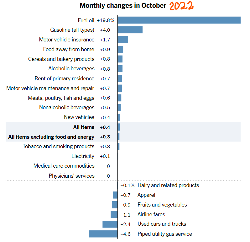
The figure below shows the main contributors to inflation in October 2022 in the USA. The inflation rate for all items was 0.4% between October and September 2022. This monthly inflation rate would correspond to annual inflation of 4.9% if the same 0.4% were verified in all following months
👉 a) If this trend continues over time, what does it tell us about the behavior of inflation?
Answer (a)
If that trend continues, it tells us that inflation was coming down (annually) in that period.
👉 b) Looking at the various items in the figure below, what items mainly contributed to the inflation rate in October 2022?
Answer (b)
The two main items that displayed a huge price increase in October were Fuel oil and Gasoline (all types). Fuel oil will affect transportation costs because almost all shipping consumes this fuel. Gasoline is the most significant energy used by everyday transportation, affecting all aspects of life.
So, if the prices of these two types of combustion items were going down to acceptable levels, overall inflation would also go down. The problem is that these prices are set in international markets, and it is unclear what individual economies can do about it.
👉 c) Can the Fed do anything to control the prices of those items most responsible for the October inflation?
Answer (c)
No, the Fed can do very little to influence the increase in Gasoline and Fuel oil prices. The Fed can reduce aggregate demand by increasing nominal interest rates and, by doing so, can reduce the demand for those items. However, the prices of oil are highly determined by a cartel (OPEC+). Therefore, the power of the Fed is quite limited in this case.
Exercise 16. New Taylor Rule: more emphasis on the output-gap
In exercise 5, we dealt with the original Taylor rule. Various economists have suggested that the original Taylor rule gives too little weight to the output gap. The (New) Taylor Rule puts a higher weight on that gap, and we will see that it performs much better than the original one. The curve has the same expression, with the only difference that now we will have
Note
The slider below Δλ_y=0.5 tells us that the central bank is more concerned about the output-gap than in the original version of the rule (where λ_y=0.5 and Δλ_y=0). See what happens by changing the value of this slider.
👉 a) Despite performing better that the original Taylor rule, what happens when extreme events knock on ecoonomic activity? Like, for example, the Great Recession of 2008-2010, the Covid pandemic in 2020, or the recent rampant inflation in 2022/20223?
Δλ_y =
Answer (a)
This New Taylor rule continues to perform poorly in the face of extreme economic events. At the bottom of the Great Recession (July 2009), it suggests that the FFR should have been negative at
These rates are impossible to justify from an economic and financial point of view.
👉 b) Given the evidence in these three rules, are monetary policy rules useless?
Answer (b)
Rules are rules; they should be used with knowledge and wisdom. Without them, a central bank may look like a ship in the open ocean without a destination. However, applying them literally shows a total lack of wisdom and prudence. The economy may be confronted by a wide range of shocks, some of which are extremely difficult to deal with given their impacts and nature.
Some rules perform poorly, but others perform very well (as seen in Exercise 6). So, if central banks base their decisions on rules that perform very well, they will make smaller mistakes than if they use bad or no rules.
But remember: no rule can accommodate all shocks that may potentially hit the economy, and no rule can work well in the face of extraordinary shocks like COVID-19 or a major war. Extraordinary shocks require extraordinary measures by central banks, and no rule can fully consider the contingencies that may arise from such situations.
Reality Check
Application 1
An important speech by Jerome Powell, Fed's Chair
Jerome Powel (2020) in a speech at the Conference “Navigating the Decade Ahead: Implications for Monetary Policy,” symposium sponsored by the Federal Reserve Bank of Kansas City, August 27, 2020, with the title "New Economic Challenges and the Fed’s Monetary Policy Review" mentioned the following:
"Inflation that runs below its desired level can lead to an unwelcome fall in longer-term inflation expectations, which, in turn, can pull actual inflation even lower, resulting in an adverse cycle of ever-lower inflation and inflation expectation.
This dynamic is a problem because expected inflation feeds directly into the general level of interest rates. Well-anchored inflation expectations are critical for giving the Fed the latitude to support employment when necessary without destabilizing inflation. But if inflation expectations fall below our 2 percent objective, interest rates would decline in tandem. In turn, we would have less scope to cut interest rates to boost employment during an economic downturn, further diminishing our capacity to stabilize the economy through cutting interest rates. We have seen this adverse dynamic play out in other major economies around the world and have learned that once it sets in, it can be very difficult to overcome. We want to do what we can to prevent such a dynamic from happening here.” (page 8/9)
Do you see any connection between what we discussed this week and the great concerns of the President (Chair) of the Federal Reserve Board of the USA in his most relevant speech in 2020? Do you think the problems of deflation and lower inflation expectations are irrelevant issues in modern macroeconomics?
Hint
This speech touches on all major points covered this week: the fear of deflation, the importance of inflation expectations, the relevance of having a 2% target interest rate, and a responsible central should do all it takes to prevent deflation from setting in.
Application 2
Ignore Japan at your peril
It is incredible how a developed, democratic, and open society fell into the deflation trap in the late 1990s, even though successive governments and central bank presidents tried to avoid such a situation. The central bank of Japan has an inflation target of 2%, like most developed economies. However, from mid-1998 until 2021, Japan could only achieve such a target in 12 out of the 264 months. In fact, most of the time, Japan has experienced quite severe deflation (-1%, -2%, and even -2.5%), some of them for extended periods. Surprisingly, despite significant deflation, the Japanese economy has displayed relatively low unemployment rates.
Can we explain this Japanese case using our model? And with our exercises above? Yes, from Exercise 8 onwards we can easily explain the Japanese case. Why has Japan not been able to escape from the long-term equilibrium inside the ZLB? Some influential economists had argued that in the past – before 2013, when Prime Minister Shinzo Abe came to power and nominated a new Governor of the Central Bank of Japan – Japanese governments and the central bank did not take the necessary measures to avoid the economy diving into the deflationary trap. They only took timid measures to deal with an exceptional danger, and the trap settled in. The positive impact on inflation of the measures taken by Prime Minister Shinzo Abe and his appointed Bank of Japan Governor (Haruhiko Kuroda) after 2013 can be easily seen in the figure above. Since 2013, the number of months with positive inflation has been much greater than those with deflation, which is a very different picture from what had happened before.
Auxiliary cells (do not delete)
Data files used in this notebook
NBER_Recessions.csv
UR_FFR.csv
EZ_inflation.csv
Taylor.csv
FFRCPIOil.csv
Scary_Paper.csv
JapanDeflationV1.csv
These CSV files must be kept in the same folder as this notebook.